Machine learning overview
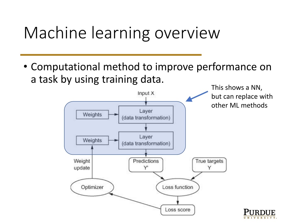


Machine learning overview
•
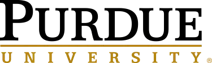
Computational method to improve performance on
a task by using training data.


This shows a NN,
but can replace with
other ML methods

Example: Linear regression
•
Task: predict
y
from
x
, using
or
Other forms possible, such as
This is still linear in the parameters
w.
•
Loss: mean squared error (MSE) between
predictions and targets


Capacity and data fitting
•
Capacity: a measure of the ability to fit complex
data
•
Increased capacity means we can make the training
error small.
•
Overfitting: like memorizing the training inputs.
Capacity large enough to reproduce training data,
but does poorly on test data. Too much capacity
for the available data.
•
Underfitting: like ignoring details. Not enough
capacity for the available detail.
Capacity and data fitting
Capacity and generalization error
Regularization
•
Sometimes minimizing the performance or loss
function directly promotes overfitting. E.g., the
Runge phenomenon of interpolating by a
polynomial using evenly spaced points.
•
Red = target function
•
Blue = degree 5
•
Green = degree 9
•
Output is linear in the coeffs
Regularization
•
Can get a better fit by using a penalty on the
coefficients. E.g.,
Example: Classification
•
Task: predict one of several classes for a given
input. E.g.,
•
Decide if a movie review is positive or negative.
•
Identify one of several possible topics for a news piece
•
Output: A probability distribution on possible
outcomes.
•
Loss: Cross-entropy (a way to compare
distributions)
Information
•
For a probability distribution p(X) for a rv X, define the
information of outcome x to be (log = nat log)
I(x) = - log p(x)
•
This is 0 if p is 1 (no information for a certain outcome)
and is large if p is near 0 (lots of information if the
event is not likely).
•
Additivity:
If X and Y are indep, then info is additive:
I(x,y) = - log p(x,y) = - log p(x)p(y) = - log p(x) - log p(y)
= I(x) + I(y)
Entropy
•
Entropy is the expected information of a rand var:
•
Note that 0 log 0 = 0
•
Entropy is a measure of
unpredictability
of a
random variable. For a given set of states, equal
probability gives maximum entropy.
Cross-entropy
•
Compare one distribution to another.
•
Suppose we have distribution p,q on same set W.
Then
•
In the discrete case,
Cross entropy as loss function
•
Question: given p(x), what q(x) minimizes the cross
entropy (in the discrete case)?
•
Constrained optimization:
Constrained optimization
•
More general constrained optimization:
•
f
is the objection function (loss)
•
g
i
are the equality constraints
•
h
j
are the inequality constraints
•
If no constraints: look for a point where gradient of
f
vanishes. But we need to include constraints.
Intuition
•
Given g = 0. Try to find points where f’ = 0 since
these points might be minima.
•
Two possibilities:
1.
We could be following a contour line of f (f does not
change along contour lines). So the contour lines of f
and g are parallel here.
2.
We have a local minimum of f (gradient of f is 0).
https://en.wikipedia.org/wiki/Lagrange_multiplier
Intuition
•
If the contours of f and g are parallel, then the
gradients of f and g are parallel. Thus we want
points (x, y) where g(x, y) = 0 and
for some λ.
•
This is the idea of Lagrange
multipliers.
https://en.wikipedia.org/wiki/Lagrange_multiplier
KKT conditions
•
Start with
•
Make the Lagrangian function
•
Take gradient and set to 0 – but other conds also.
KKT conditions
•
Make the Lagrangian function
•
Necessary conditions to have a minimum are
Cross entropy
•
Exercise for the reader: Use the KKT conditions to
show that if
p
i
are fixed, positive, and sum to 1,
then the
q
i
that solves
is
q
i
=
p
i
.
That is,
Regularization and constraints
•
Regularization is something like a weak constraint.
•
E.g., for L
2
penalty, instead of requiring the weights
to be small with a penalty like <
c
we just
prefer them to be small by adding to the
objective function.
Enhance task performance by leveraging training data with a focus on neural networks and other machine learning techniques. Explore the use of computational methods to boost accuracy and efficiency in completing tasks.

Download Presentation

Please find below an Image/Link to download the presentation.
The content on the website is provided AS IS for your information and personal use only. It may not be sold, licensed, or shared on other websites without obtaining consent from the author.If you encounter any issues during the download, it is possible that the publisher has removed the file from their server.
You are allowed to download the files provided on this website for personal or commercial use, subject to the condition that they are used lawfully. All files are the property of their respective owners.
The content on the website is provided AS IS for your information and personal use only. It may not be sold, licensed, or shared on other websites without obtaining consent from the author.
E N D
Presentation Transcript
Machine learning overview Computational method to improve performance on a task by using training data. This shows a NN, but can replace with other ML methods
Example: Linear regression Task: predict y from x, using or Other forms possible, such as This is still linear in the parameters w. Loss: mean squared error (MSE) between predictions and targets
Capacity and data fitting Capacity: a measure of the ability to fit complex data Increased capacity means we can make the training error small. Overfitting: like memorizing the training inputs. Capacity large enough to reproduce training data, but does poorly on test data. Too much capacity for the available data. Underfitting: like ignoring details. Not enough capacity for the available detail.
Regularization Sometimes minimizing the performance or loss function directly promotes overfitting. E.g., the Runge phenomenon of interpolating by a polynomial using evenly spaced points. Red = target function Blue = degree 5 Green = degree 9 Output is linear in the coeffs
Regularization Can get a better fit by using a penalty on the coefficients. E.g.,
Example: Classification Task: predict one of several classes for a given input. E.g., Decide if a movie review is positive or negative. Identify one of several possible topics for a news piece Output: A probability distribution on possible outcomes. Loss: Cross-entropy (a way to compare distributions)
Information For a probability distribution p(X) for a rv X, define the information of outcome x to be (log = nat log) I(x) = - log p(x) This is 0 if p is 1 (no information for a certain outcome) and is large if p is near 0 (lots of information if the event is not likely). Additivity: If X and Y are indep, then info is additive: I(x,y) = - log p(x,y) = - log p(x)p(y) = - log p(x) - log p(y) = I(x) + I(y)
Entropy Entropy is the expected information of a rand var: Note that 0 log 0 = 0 Entropy is a measure of unpredictability of a random variable. For a given set of states, equal probability gives maximum entropy.
Cross-entropy Compare one distribution to another. Suppose we have distribution p,q on same set W. Then In the discrete case,
Cross entropy as loss function Question: given p(x), what q(x) minimizes the cross entropy (in the discrete case)? Constrained optimization:
Constrained optimization More general constrained optimization: f is the objection function (loss) giare the equality constraints hjare the inequality constraints If no constraints: look for a point where gradient of f vanishes. But we need to include constraints.
Intuition Given g = 0. Try to find points where f = 0 since these points might be minima. Two possibilities: 1. We could be following a contour line of f (f does not change along contour lines). So the contour lines of f and g are parallel here. 2. We have a local minimum of f (gradient of f is 0). https://en.wikipedia.org/wiki/Lagrange_multiplier
Intuition If the contours of f and g are parallel, then the gradients of f and g are parallel. Thus we want points (x, y) where g(x, y) = 0 and for some . This is the idea of Lagrange multipliers. https://en.wikipedia.org/wiki/Lagrange_multiplier
KKT conditions Start with Make the Lagrangian function Take gradient and set to 0 but other conds also.
KKT conditions Make the Lagrangian function Necessary conditions to have a minimum are
Cross entropy Exercise for the reader: Use the KKT conditions to show that if piare fixed, positive, and sum to 1, then the qi that solves is qi = pi.That is,
Regularization and constraints Regularization is something like a weak constraint. E.g., for L2 penalty, instead of requiring the weights to be small with a penalty like < c we just prefer them to be small by adding to the objective function.