Machine Learning Methods on 2D Ising Model


Many important works
Many important works
arise in this category
arise in this category
•
Input vecto
Input vecto
r
r
•
Output vecto
Output vecto
r
r
•
Weighting matrices to be learnt
Weighting matrices to be learnt
•
3
3
-layer Neural Network.
-layer Neural Network.
•
1 input layer
1 input layer
•
1 hidden layer
1 hidden layer
•
1 output layer
1 output layer
Data flows forward into the network
Data flows forward into the network
Gradient of Error flows backward to
Gradient of Error flows backward to
each layer
each layer
The network “Learns” using
The network “Learns” using
Stochastic gradient descent
Stochastic gradient descent
Underfitting happens when the network doesn’t do well on
Underfitting happens when the network doesn’t do well on
both training and testing set.
both training and testing set.
Overfitting happens when the network does well on training
Overfitting happens when the network does well on training
set but not well on testing set.
set but not well on testing set.
An
An
EPOCH
EPOCH
is the action of passing all the data
is the action of passing all the data
into the network
into the network
A
A
BATCH
BATCH
is the number of data fed into the
is the number of data fed into the
network at once, and back-propagation is
network at once, and back-propagation is
performed.
performed.
A smaller batch size reduces overfitting as the
A smaller batch size reduces overfitting as the
batch is “noisier”
batch is “noisier”
The two-dimensional square-lattice Ising model is one of the simplest
The two-dimensional square-lattice Ising model is one of the simplest
models to show a phase transition.
models to show a phase transition.
Monte Carlo simulation can be used to generate the configurations of
Monte Carlo simulation can be used to generate the configurations of
Ising model at different temperatures
Ising model at different temperatures
See Lecture note 11 for more details
See Lecture note 11 for more details
Transfer Probability
Far below
Far below
the
the
critical
critical
temperature
temperature
Slightly below
Slightly below
the
the
critical
critical
temperature
temperature
Near
Near
the critical
the critical
temperature
temperature
Far above
Far above
the
the
critical
critical
temperature
temperature
Slightly above
Slightly above
the
the
critical
critical
temperature
temperature
Potential application: interpretation of in-situ measurement.
Potential application: interpretation of in-situ measurement.
For example, during crystal growth, difficult to measure the
For example, during crystal growth, difficult to measure the
temperature of growth front.
temperature of growth front.
A combination of Monte Carlo and Machine learning can give direct
A combination of Monte Carlo and Machine learning can give direct
interpretation of the experimental morphology.
interpretation of the experimental morphology.
Accurate control and tuning become possible.
Accurate control and tuning become possible.
2.26
2.26
4.2
4.2
……
……
……
……
0.8
0.8
Save in an 30000-sizes array
Save in an 30000-sizes array
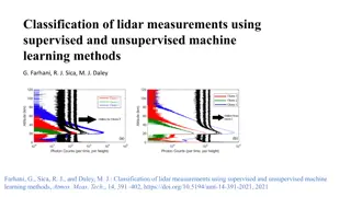
We did Monte Carlo simulation at five different temperatures with 6000 samples each.
We did Monte Carlo simulation at five different temperatures with 6000 samples each.
Random initial configurations and 100000 MC steps, so they are likely to reach equilibrium.
Random initial configurations and 100000 MC steps, so they are likely to reach equilibrium.
Training
Training
Group
Group
No
No
Yes
Yes
Any slides with the
Any slides with the
★
★
symbol means there’s
symbol means there’s
something you can
something you can
modify for your project
modify for your project
★
Insert Extra Layers here
★
★
Example: 4 label case
Example: 4 label case
★
★
★
★
Change the following settings of the machine learning model to make the accuracy higher than
Change the following settings of the machine learning model to make the accuracy higher than
95%
95%
1.
Activation Function
Activation Function
2.
Learning rate
Learning rate
3.
Batch Size
Batch Size
4.
Number of Layers (But no larger than
Number of Layers (But no larger than
10
10
)
)
5.
Number of Epochs (But no larger than
Number of Epochs (But no larger than
10
10
)
)
6.
Less than
Less than
20
20
neurons per layer
neurons per layer
7.
Avoid Overfitting ( less than
Avoid Overfitting ( less than
5%
5%
difference in accuracy between training and testing )
difference in accuracy between training and testing )
Submit your .ipynb file with a short readme about your result
Submit your .ipynb file with a short readme about your result
Our Result:
Key concepts in machine learning and the application of neural networks to infer temperature based on spin configurations of the Ising model.

Download Presentation

Please find below an Image/Link to download the presentation.
The content on the website is provided AS IS for your information and personal use only. It may not be sold, licensed, or shared on other websites without obtaining consent from the author.If you encounter any issues during the download, it is possible that the publisher has removed the file from their server.
You are allowed to download the files provided on this website for personal or commercial use, subject to the condition that they are used lawfully. All files are the property of their respective owners.
The content on the website is provided AS IS for your information and personal use only. It may not be sold, licensed, or shared on other websites without obtaining consent from the author.
E N D
Presentation Transcript
Machine Learning Methods on 2D Ising Model
Todays content Brief Review of Key concepts in Machine learning Inversely infer temperature based on spin configurations of Ising model with neural network.
Introduction on Machine Learning Machine learning (ML) is the study of computer algorithms that can improve automatically through experience. Three broad categories: Supervised Learning: Label are given as desired outputs, and it is to learn a general rule that maps inputs to outputs. Examples: - Classification: (category) digits recognition Animal identification - Regression: (real value) House prices prediction
Introduction on Machine Learning Unsupervised Learning: No labels are given to the learning algorithm, leaving it on its own to find structure in its input. Examples: - Clustering just by the distribution of the data, the computer has no knowledge of the labels Reinforcement Learning: A computer program interacts with a dynamic environment in which it must perform a certain goal (A game-like situation) Reinforcement Learning is often mixed with Unsupervised Learning Examples: - autonomous vehicle -OpenAI Five (Dota 2) -AlphaGo Zero Many important works arise in this category
Machine Learning Frameworks Pytorch, TensorFlow, Keras are the most popular machine learning packages Python is the most convenient programming language for Machine learning Google Colab provides preinstalled python environments
Example : Fully Connected Neural Network x y Input vector Output vector W Weighting matrices to be learnt Some nonlinear function (activations) Sigmoid Tanh ReLU etc... 3-layer Neural Network. 1 input layer 1 hidden layer 1 output layer
Activation Functions Multiple activation functions available Sigmoid and RELU: the most common
The Forward And backward Pass Data flows forward into the network Gradient of Error flows backward to each layer The network Learns using Stochastic gradient descent
Overfitting and Underfitting Underfitting happens when the network doesn t do well on both training and testing set. Overfitting happens when the network does well on training set but not well on testing set.
Fitting Data into the network An EPOCH is the action of passing all the data into the network A BATCH is the number of data fed into the network at once, and back-propagation is performed. A smaller batch size reduces overfitting as the batch is noisier
Application of machine learning in physical system Inversely infer temperature based on spin configurations of ising model with neuron network.
Back to Ising model The two-dimensional square-lattice Ising model is one of the simplest models to show a phase transition. Monte Carlo simulation can be used to generate the configurations of Ising model at different temperatures See Lecture note 11 for more details Transfer Probability To simplify the model, just set ? = 1; = 0;??= 1
Ising Model vs. Temperature T represent Far below the critical temperature temperature (unit: K ?? ?? 1) ? is the average Slightly below the critical temperature magnetic moment (unit: ?J) Near the critical temperature Slightly above the critical temperature Far above the critical temperature
Inversely infer simulation condition of Ising Model Monte Carlo Simulation of Ising Model Equilibrium configuration Temperature Machine learning
Importance of such simulations Potential application: interpretation of in-situ measurement. For example, during crystal growth, difficult to measure the temperature of growth front. A combination of Monte Carlo and Machine learning can give direct interpretation of the experimental morphology. Accurate control and tuning become possible.
General Model Input Layer What should be used as the input layer? Neural Network Output Layer Range of temperature. It is challenging to give accurate prediction of the exact temperature Possible to distinguish a few most probable temperature ranges. To simplify the problem, we offer training data of 5 most probable temperatures and your neural network should give predictions of the temperature based on the spin morphology.
Input data We did Monte Carlo simulation at five different temperatures with 6000 samples each. Random initial configurations and 100000 MC steps, so they are likely to reach equilibrium. 6000 6000 6000 6000 6000 Configurations in T=4.2 Configurations in T=2.4 Configurations in T=2.26 Configurations in T=0.8 Configurations in T=2.1 Mix and Shuffle 30000 Configurations X_tes Save in 30000 30 30 matrices consisting of 1 and 1 Training Group Corresponding temperature 2.26 4.2 0.8 Y_tes Save in an 30000-sizes array
Output Requirement You need to exactly predict the corresponding most probable temperature range of the configurations in the test set. These are the five labels Far below the critical temperature Slightly below the critical temperature Near the critical temperature Slightly above the critical temperature Far above the critical temperature
Flow chart Input the configuration and corresponding temperature Divide the data into training group and testing group Set up the learning model (layer, epochs, batch size, activation functions, learning rate ) Any slides with the symbol means there s something you can modify for your project No Training Calculation accuracy for the testing group Yes Accurate enough? End
Development environment Python with Tensorflow : Keras High-level package based on Python Easy to use and learn, straightforward Very good online documentation Like any Python package, you need to import it!
Simple Sequential Model with Keras Sequential Neural Network From up to down , executed in order, layer-by-layer You can freely append layers to the list
Handling Input data with Keras Define an input shape of the data you want to put into the model Define an input layer , and a Flatten layer You do not need to touch this code, just understand what it s doing When you add layers, do it AFTER the input layer and flatten layer Insert Extra Layers here
What does this model do? Feeds in (30,30) matrix Flattens into 900 elements array, the input layer and flatten layer has no trainable parameters Passes through one hidden layer of Sigmoid neurons, output a 100 elements array Outputs 5 numbers
What doesnt this model do (yet)? Learn! It s only a mechanism that turns matrices into 5 numbers Use the compile method to specify the optimizer and cost function You can choose the learning rate Cost Function will be fixed to Sparse Categorical Cross-entropy
The Cost Function Categorical CrossEntropy is designed to process classification results Example: 4 label case The perfect model should have the CrossEntropy (Loss) of 0 The network will try to minimize the Loss by Stochastic gradient descend
Feeding the data forward Feeding the training data into the network The fit method selects data to be used as input or as answer Configure the batch_size and epochs in this method
Dense Layers with Keras Dense Layer can contain arbitrary number (chosen by the user) of sigmoid (or other activation function) neurons! Example : layer with 20 sigmoid neurons You can set the number of neurons and the activation function of every layer
Choosing Optimizers Simple method: In the compile method, choose by the name of the optimizer Advanced Method: Choose using an instance to specify the learning rate as shown In today s lab, the optimizer is fixed to be Adam
Choosing Batch size and Epoch Batch Size batch_size Defines the number of samples in a mini-batch of the training set Larger batch will have better estimate on the error Smaller batches might converge faster with some noise It s limited by the total amount of data in the training set Epochs epochs Defines the number of epochs to train the network with The network will eventually converge to some minima (local or global) , so more isn t always better! You ll be limited to 10 Epochs in this lab
Evaluate your model Just like you, your model need to take exams too Fortunately, it s easy ( for you ) This is how you check the accuracy of this model, make sure to use the TESTING SET as input when you check it ! You ll be GRADED with the result of the evaluation of your model
How to do? Open Google Collab and load database Set up your own machine learning model Train and test Calculation accuracy for discrete test group
Requirement Change the following settings of the machine learning model to make the accuracy higher than 95% 1. Activation Function 2. Learning rate 3. Batch Size 4. Number of Layers (But no larger than 10) 5. Number of Epochs (But no larger than 10) 6. Less than 20 neurons per layer 7. Avoid Overfitting ( less than 5% difference in accuracy between training and testing ) Submit your .ipynb file with a short readme about your result Our Result:


?")