Long-Run Cost Curves

7c – Long Run Cost Curves
This web quiz may appear as two pages on
tablets and laptops.
I recommend that you view it as one page by
clicking on the open book icon at the
bottom of the page.


Lesson 7a – The Production Function
How output changes as we add more resources (workers)
Lesson 7b – Short Run Costs
How costs change as we produce more output in the
same factory
Lesson 7c – Long Run Costs
How costs change in the long run as we produce more
output in larger factories

7b Review – Short Run Costs
•
TC
•
TVC
•
TFC
•
ATC
•
AVC
•
AFC
•
and MC
Be able to:
•
Calculate
•
Define
•
Draw
•
Describe graph shapes
•
Give Examples
7b Review - Short Run Cost Curves
Short Run Cost Curves
Be able to find:
•
TC
•
TVC
•
TFC
•
ATC
•
AVC
•
AFC
•
MC
On a:
•
Table of data (YP 35, 45)
•
Graph with numbers
(YP 38-39)
•
Graph with letters using
geometry (YP 44)
Do:
-
7b Yellow Pages
-
7b Web Quiz
-
7b Clicker quiz
7b Review - Short Run Cost Curves
Total Cost Curves Average Cost Curves
and MC
7b Review - Short Run Cost Curves
The profit max. Q is where MR = MC, therefore the rent paid is
irrelevant to the question "should we produce more?“. Higher
rent does not change the MC. “Ignore fixed costs”.
7b Review - Short Run Cost Curves
Outcomes / What you should know:
•
Explain the difference between short run and long
run costs
•
State why the long run average cost is expected to
be U shaped
•
List and explain the causes of economies and
diseconomies of scale
•
Indicate the relationship between economies of
scale and number of firms in an industry and their
sizes
•
Why are there many hardware stores in Illinois but
only two automobile production plants?
7c – Long Run Costs
Key Terms
short run,
long run,
economies of scale,
diseconomies of scale,
constant returns to scale,
minimum efficient scale,
natural monopoly
7c – Long Run Costs
Introduction
•
In lesson 7b we calculated and graphed SHORT
RUN costs when the size of the factory was fixed
(did not change). Here we will learn how costs
change in the LONG RUN.
In the long run we can
change the size of the factory. Only in the long
run can new firms enter an industry and only in
the long run can firms leave the industry (go out
of business).
Be sure that you can define "short
run" and "long run".
•
As always, be sure you know why the long run ATC
curve has the shape it does; For all graphs:
DEFINE, DRAW, DESCRIBE the shape.
•
Note that in the next unit (unit 3) we will use long
run graphs to find the allocatively efficient
quantity and the productively efficient quantity.
7c – Long Run Costs
Something Interesting – Why are we
studying this?
•
Why are there many
hardware stores in
Illinois but only two
automobile production
plants?
•
ANSWER: The answer
has to do with the
different shapes of the
long run ATC curve for
retail stores and for
automobile production.
7c – Long Run Costs
1. In the long run, which
is NOT true?
1.
All inputs are variable
2.
There are no fixed costs
3.
The firm can change the size of its factory
4.
The only fixed costs are from long term leases
1. In the long run, which
is NOT true?
1.
All inputs are variable
2.
There are no fixed costs
3.
The firm can change the size of its factory
4.
The only fixed costs are from long term leases
2. Which is a long run
change?
1.
Hiring more workers
2.
Shutting down for three weeks
3.
Going out of business
4.
Increasing advertising
2. Which is a long run
change?
1.
Hiring more workers
2.
Shutting down for three weeks
3.
Going out of business
4.
Increasing advertising
3. To produce
an output of 30
in the long run,
what size
factory should
be used?
YP 50
1.
A
2.
B
3.
C
4.
Can’t tell
3. To produce an
output of 30 in
the long run,
what size factory
should be used?
YP 50
1.
A
2.
B
3.
C
4.
Can’t tell
7c – Long Run Costs
7c – Long Run Costs
7c – Long Run Costs
For ALL graphs:
•
Define
•
Draw
•
Describe the shape
4. Economies
of scale occur
between
______;
Disecon. Of
scale occur
between
_____. YP 50
1.
10-30; 30-100
2.
10-40; 40-100
3.
10-50; 50-100
4.
10-70; 70-100
4. Economies
of scale occur
between
______;
Disecon. Of
scale occur
between
_____. YP 50
1.
10-30; 30-100
2.
10-40; 40-100
3.
10-50; 50-100
4.
10-70; 70-100
NOTE - in the video lectures:
•
Economies of scale = increasing returns to scale
•
Diseconomies of scale = decreasing returns to scale
ECONOMIES OF SCALE
Explanation:
Reductions in the average total cost of producing a
product as the firm expands the size of plant (its output) in the long
run; the economies of mass production.
Rationale:
(1) labor specialization
(2) managerial specialization
(3) productively efficient use of capital
(4) other factors: such as design, development, or other "start up"
costs such as advertising and "learning by doing."
7c – Long Run Costs
DISECONOMIES OF SCALE
Explanation:
Increase in the average total cost of producing a
product as the firm expands the size of its plant (its output) in the
long run.
Rationale:
some reasons include distant management, worker
alienation, and problems with communication and coordination.
7c – Long Run Costs
CONSTANT RETURNS TO SCALE
Explanation:
A situation wherein long-run average cost does
not change. A given percentage increase in
all
outputs will
cause a proportionate percentage increase in output.
In this range, ATC remains constant. (Between Q1 and Q3
below)
7c – Long Run Costs
5. What causes
diseconomies of scale?
1.
Specialization of labor
2.
Teamwork
3.
Management problems
4.
More efficient use of capital
5. What causes
diseconomies of scale?
1.
Specialization of labor
2.
Teamwork
3.
Management problems
4.
More efficient use of capital
6. If output increases from 10
to 15 when a firm doubles all
of its inputs then this firm has:
1.
Economies of (increasing returns to) scale
2.
Diseconomies of (decreasing returns to) scale
3.
Constant returns to scale
4.
A downward sloping long run ATC curve
6. If output increases from 10
to 15 when a firm doubles all
of its inputs then this firm has:
1.
Economies of (increasing returns to) scale
2.
Diseconomies of (decreasing returns to) scale
3.
Constant returns to scale
4.
A downward sloping long run ATC curve
7. Minimum
efficient scale
occurs at:
1.
Q1
2.
Q2
3.
Q3
4.
Can’t tell
7. Minimum
efficient scale
occurs at:
1.
Q1
2.
Q2
3.
Q3
4.
Can’t tell
Do YP 48
7c – Long Run Costs
8. Which represents an industry
with small and large firms?
1.
A
2.
B
3.
C
8. Which represents an industry
with small and large firms?
1.
A
2.
B
3.
C
9. Which represents the car industry?
1.
A
2.
B
3.
C
9. Which represents the car industry?
1.
A
2.
B
3.
C
10. To maximize profits,
firms will produce the
quantity where:
1.
MSB=MSC
2.
LR-ATC is at a minimum
3.
TR is at a maximum
4.
MR = MC
10. To maximize profits,
firms will produce the
quantity where:
1.
MSB=MSC
2.
LR-ATC is at a minimum
3.
TR is at a maximum
4.
MR = MC
To
maximize profits
businesses will
produce the quantity where:
MR = MC
This means they will produce:
•
All
where MR > MC
•
Up to where MR = MC
Differences between short run and long run costs, learn about economies and diseconomies of scale, and understand the relationship between scale and firm size in various industries. Key terms include short run, long run, economies of scale, and natural monopoly.

Download Presentation

Please find below an Image/Link to download the presentation.
The content on the website is provided AS IS for your information and personal use only. It may not be sold, licensed, or shared on other websites without obtaining consent from the author. Download presentation by click this link. If you encounter any issues during the download, it is possible that the publisher has removed the file from their server.
E N D
Presentation Transcript
7c Long Run Cost Curves This web quiz may appear as two pages on tablets and laptops. I recommend that you view it as one page by clicking on the open book icon at the bottom of the page.
7b Review Short Run Costs Lesson 7a The Production Function How output changes as we add more resources (workers) Lesson 7b Short Run Costs How costs change as we produce more output in the same factory Lesson 7c Long Run Costs How costs change in the long run as we produce more output in larger factories
Short Run Cost Curves TC TVC TFC ATC AVC AFC and MC Be able to: Calculate Define Draw Describe graph shapes Give Examples 7b Review - Short Run Cost Curves
Be able to find: TC TVC TFC ATC AVC AFC MC On a: Table of data (YP 35, 45) Graph with numbers (YP 38-39) Graph with letters using geometry (YP 44) Do: - - - 7b Yellow Pages 7b Web Quiz 7b Clicker quiz 7b Review - Short Run Cost Curves
Total Cost Curves Average Cost Curves and MC 7b Review - Short Run Cost Curves
The profit max. Q is where MR = MC, therefore the rent paid is irrelevant to the question "should we produce more? . Higher rent does not change the MC. Ignore fixed costs . 7b Review - Short Run Cost Curves
7c Long Run Costs Outcomes / What you should know: Explain the difference between short run and long run costs State why the long run average cost is expected to be U shaped List and explain the causes of economies and diseconomies of scale Indicate the relationship between economies of scale and number of firms in an industry and their sizes Why are there many hardware stores in Illinois but only two automobile production plants?
Key Terms short run, long run, economies of scale, diseconomies of scale, constant returns to scale, minimum efficient scale, natural monopoly 7c Long Run Costs
Introduction In lesson 7b we calculated and graphed SHORT RUN costs when the size of the factory was fixed (did not change). Here we will learn how costs change in the LONG RUN. In the long run we can change the size of the factory. Only in the long run can new firms enter an industry and only in the long run can firms leave the industry (go out of business). Be sure that you can define "short run" and "long run". As always, be sure you know why the long run ATC curve has the shape it does; For all graphs: DEFINE, DRAW, DESCRIBE the shape. Note that in the next unit (unit 3) we will use long run graphs to find the allocatively efficient quantity and the productively efficient quantity. 7c Long Run Costs
Something Interesting Why are we studying this? Why are there many hardware stores in Illinois but only two automobile production plants? ANSWER: The answer has to do with the different shapes of the long run ATC curve for retail stores and for automobile production. 7c Long Run Costs
1. In the long run, which is NOT true? 1. All inputs are variable 2. There are no fixed costs 3. The firm can change the size of its factory 4. The only fixed costs are from long term leases
1. In the long run, which is NOT true? 1. All inputs are variable 2. There are no fixed costs 3. The firm can change the size of its factory 4. The only fixed costs are from long term leases
2. Which is a long run change? 1. Hiring more workers 2. Shutting down for three weeks 3. Going out of business 4. Increasing advertising
2. Which is a long run change? 1. Hiring more workers 2. Shutting down for three weeks 3. Going out of business 4. Increasing advertising
3. To produce an output of 30 in the long run, what size factory should be used? YP 50 1. A 2. B 3. C 4. Can t tell
3. To produce an output of 30 in the long run, what size factory should be used? YP 50 1. A 2. B 3. C 4. Can t tell
For ALL graphs: Define Draw Describe the shape 7c Long Run Costs
4. Economies of scale occur between ______; Disecon. Of scale occur between _____. YP 50 1. 10-30; 30-100 2. 10-40; 40-100 3. 10-50; 50-100 4. 10-70; 70-100
4. Economies of scale occur between ______; Disecon. Of scale occur between _____. YP 50 1. 10-30; 30-100 2. 10-40; 40-100 3. 10-50; 50-100 4. 10-70; 70-100
NOTE - in the video lectures: Economies of scale = increasing returns to scale Diseconomies of scale = decreasing returns to scale
ECONOMIES OF SCALE Explanation: Reductions in the average total cost of producing a product as the firm expands the size of plant (its output) in the long run; the economies of mass production. Rationale: (1) labor specialization (2) managerial specialization (3) productively efficient use of capital (4) other factors: such as design, development, or other "start up" costs such as advertising and "learning by doing." 7c Long Run Costs
DISECONOMIES OF SCALE Explanation: Increase in the average total cost of producing a product as the firm expands the size of its plant (its output) in the long run. Rationale: some reasons include distant management, worker alienation, and problems with communication and coordination. 7c Long Run Costs
CONSTANT RETURNS TO SCALE Explanation: A situation wherein long-run average cost does not change. A given percentage increase in all outputs will cause a proportionate percentage increase in output. In this range, ATC remains constant. (Between Q1 and Q3 below) 7c Long Run Costs
5. What causes diseconomies of scale? 1. Specialization of labor 2. Teamwork 3. Management problems 4. More efficient use of capital
5. What causes diseconomies of scale? 1. Specialization of labor 2. Teamwork 3. Management problems 4. More efficient use of capital
6. If output increases from 10 to 15 when a firm doubles all of its inputs then this firm has: 1. Economies of (increasing returns to) scale 2. Diseconomies of (decreasing returns to) scale 3. Constant returns to scale 4. A downward sloping long run ATC curve
6. If output increases from 10 to 15 when a firm doubles all of its inputs then this firm has: 1. Economies of (increasing returns to) scale 2. Diseconomies of (decreasing returns to) scale 3. Constant returns to scale 4. A downward sloping long run ATC curve
7. Minimum efficient scale occurs at: 1. Q1 2. Q2 3. Q3 4. Can t tell
7. Minimum efficient scale occurs at: 1. Q1 2. Q2 3. Q3 4. Can t tell
7c Long Run Costs Do YP 48
8. Which represents an industry with small and large firms? 1. A 2. B 3. C
8. Which represents an industry with small and large firms? 1. A 2. B 3. C
9. Which represents the car industry? 1. A 2. B 3. C
9. Which represents the car industry? 1. A 2. B 3. C
10. To maximize profits, firms will produce the quantity where: 1. MSB=MSC 2. LR-ATC is at a minimum 3. TR is at a maximum 4. MR = MC
10. To maximize profits, firms will produce the quantity where: 1. MSB=MSC 2. LR-ATC is at a minimum 3. TR is at a maximum 4. MR = MC
To maximize profits businesses will produce the quantity where: MR = MC This means they will produce: All where MR > MC Up to where MR = MC