Logistic Regression with “Grouped” Data

Logistic Regression with “Grouped” Data
Lobster Survival by Size in a Tethering
Experiment
Source: E.B. Wilkinson, J.H. Grabowski, G.D. Sherwood, P.O. Yund (2015). "Influence of Predator
Identity on the Strength of Predator Avoidance Response in Lobsters," Journal of Experimental
Biology and Ecology, Vol. 465, pp. 107-112.

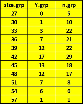
Data Description
•
Experiment involved 159 juvenile lobsters in a Saco
Bay, Maine
•
Outcome: Whether or not lobster survived predator
attack in Tethering Experiment
•
Predictor Variable: Length of Carapace (mm).
Lobsters grouped in
m
= 11 groups of width of 3mm (27 to
57 by 3)

Models
•
Data: (Y
i
,n
i
) i=1,…,m
•
Distribution: Binomial at each Size Level (X
i
)
•
Link Function: Logit: log(
i
/(1-
i
)) is a linear function of
Predictor (Size Level)
•
3 Possible Linear Predictors:
log(
i
/(1-
i
)) =
(Mean is same for all Sizes, No association)
log(
i
/(1-
i
)) =
X
i
(Linearly related to size)
log(
i
/(1-
i
)) =
Z
1
+…+
m-1
Z
m-1
+
m
Z
m
Z
i
= 1 if Size Level i, 0
o.w. This allows for m distinct logits, without a linear trend in
size (aka Saturated model)
Probability Distribution & Likelihood Function - I
Maximum Likelihood Estimation – Model 1
Maximum Likelihood Estimation – Model 3
Model 2 – R Output
glm(formula = lob.y ~ size, family = binomial("logit"))Coefficients:
Estimate Std. Error z value Pr(>|z|)
(Intercept) -7.89597 1.38501 -5.701 1.19e-08 ***
size 0.19586 0.03415 5.735 9.77e-09 ***
Evaluating the log-likelihood for Different Models
Deviance and Likelihood Ratio Tests
•
Deviance:
-2*(log Likelihood of Model – log Likelihood of Saturated Model)
Degrees of Freedom = # of Parameters in Saturated Model - # in
model
•
When comparing a Complete and Reduced Model, take
difference between the Deviances (Reduced – Full)
•
Under the null hypothesis, the statistic will be chi-square
with degrees of freedom = difference in degrees of
freedoms for the 2 Deviances (number of restrictions
under null hypothesis)
•
Deviance can be used to test goodness-of-fit of model.
Deviance and Likelihood Ratio Tests
Pearson Chi-Square Test for Goodness-of-Fit
Pearson Chi-Square Test for Goodness-of-Fit
Even though some of the group sample sizes are small, and some Expected cell
Counts are below 5, it is clear that Model 2 provides a Good Fit to the data
Residuals
Residuals
Computational Approach for ML Estimator
Estimated Variance-Covariance for ML Estimator
ML Estimate, Variance, Standard Errors
> mod2 <- glm(lob.y ~ size, family=binomial("logit"))> summary(mod2)
Call: glm(formula = lob.y ~ size, family = binomial("logit"))Deviance Residuals:
Min 1Q Median 3Q Max
-1.12729 -0.43534 0.04841 0.29938 1.02995
Coefficients:
Estimate Std. Error z value Pr(>|z|)
(Intercept) -7.89597 1.38501 -5.701 1.19e-08 ***
size 0.19586 0.03415 5.735 9.77e-09 ***
Null deviance: 52.1054 on 10 degrees of freedom
Residual deviance: 4.5623 on 9 degrees of freedom
AIC: 32.24
logLik(mod2)
'log Lik.' -14.11992 (df=2)
Logistic regression analysis was performed to investigate how predator identity influences lobster survival by size in a tethering experiment. The study by Wilkinson et al. (2015) delved into the dynamics of predator avoidance responses in lobsters. Results shed light on the complex interactions between lobsters and predators in their environment, offering valuable insights for ecological research and management strategies.

Download Presentation

Please find below an Image/Link to download the presentation.
The content on the website is provided AS IS for your information and personal use only. It may not be sold, licensed, or shared on other websites without obtaining consent from the author.If you encounter any issues during the download, it is possible that the publisher has removed the file from their server.
You are allowed to download the files provided on this website for personal or commercial use, subject to the condition that they are used lawfully. All files are the property of their respective owners.
The content on the website is provided AS IS for your information and personal use only. It may not be sold, licensed, or shared on other websites without obtaining consent from the author.
E N D
Presentation Transcript
Logistic Regression with Grouped Data Lobster Survival by Size in a Tethering Experiment Source: E.B. Wilkinson, J.H. Grabowski, G.D. Sherwood, P.O. Yund (2015). "Influence of Predator Identity on the Strength of Predator Avoidance Response in Lobsters," Journal of Experimental Biology and Ecology, Vol. 465, pp. 107-112.
Data Description Experiment involved 159 juvenile lobsters in a Saco Bay, Maine Outcome: Whether or not lobster survived predator attack in Tethering Experiment Predictor Variable: Length of Carapace (mm). Lobsters grouped in m = 11 groups of width of 3mm (27 to 57 by 3) size.grp 27 30 33 36 39 42 45 48 51 54 57 Y.grp 0 1 3 7 12 17 13 12 7 6 1 n.grp 5 10 22 21 22 29 18 17 8 6 1 79 159 m m ^ = = = = Overall: 79 159 0.4969 Y n i i = = 1 1 i i
Models Data: (Yi,ni) i=1, ,m Distribution: Binomial at each Size Level (Xi) Link Function: Logit: log( i/(1- i)) is a linear function of Predictor (Size Level) 3 Possible Linear Predictors: log( i/(1- i)) = (Mean is same for all Sizes, No association) log( i/(1- i)) = + Xi(Linearly related to size) log( i/(1- i)) = Z1 + + m-1Zm-1 + mZm o.w. This allows for m distinct logits, without a linear trend in size (aka Saturated model) Zi= 1 if Size Level i, 0 f = 1 e e + = = Note for a linear predictor for the logit link: log f + f f 1 1 1 e
Probability Distribution & Likelihood Function - I n y ! n n ( ) ( ) ( ) ( ) n y n y i = = y y ~ , | , 1 1 0 i Y Bin n f y n y n i i i i i i ( ) i i i i i i i i i i i i ! ! y y i i i n n i ! m ( ) ( ) n y = y Assuming independence among the : ,..., 1 i y f y y i i i ( ) 1 i m i i ! ! y y = 1 i i i i Consider 3 Models for : i = = = e + = Model 1: log i i 1 1 e i + X e + i + = Model 2: log i X i i + X 1 1 e i i 1 1 Z + + + 1 if Size Group i 0 otherwise ... Z Z e 1 1 m m m m + + + = = Model 3: log ... where i Z Z Z Z 1 1 1 1 m m m m i i 1 1 Z + + m m + ... Z Z 1 + 1 1 m m 1 e i We can consider the distribution function as a Likelihood function for the regression coefficients given the data ,..., ! 1 ! ! i i i i y n y = 1 1 For Model 3: ,..., , m m : y y 1 m m n ( ) ( ) n y = y i L i i i ( ) i i 1 For Model 1: For Model 2: ,
Maximum Likelihood Estimation Model 1 = 1 e + = = Model 1: log 1 i i i + 1 1 1 e e i y i ! ! ! m m m n n n n n n )( ) ( ! ) y n ( ) ( ) ( ) n y n = = = + = y i i 1 1 1 i i i i L e e i i i i ( ) ( ) ( i i i ! ! ! ! 1 ! y y y y han the Likelihood y y = = = 1 1 1 i i i i i i i i i i i i i The log-Likelihood typically is easier to maximize t ( ) 1 We maximize Likelihood by differentiating log likelihood, setting it to zero, and solving for unknown parameters ( ) ( ) ( ) ( ( 1 i = m ( ) ( ) ( ) ( ) ( ) ( ) ( ) ( ) ( ) ( ) ( ) = = + + log log ! log ! log ! log log 1 log 1 l L n y n y y n i i i i i i i i i = i ( ) m ( ) e ( ) ) ( ) ( ) ) = = + + = log log ! log ! log ! log log 1 l L n y n y y n e i i i i i i m ( ) ( ) ( ) ( ) ( ) + i + log ! log ! log ! log 1 n y n y y n e i i i i i = 1 i m n ^ ( ) ( ) ^ log L + i 1 1 m m m e + e e set = = = = + = = 0 1 1 i y n y n i i i i ^ ^ m ^ 1 e + 1 e = = = 1 1 1 i i i y e e i = 1 i m m m m m n y y y y i i i i i ^ 1 79 159 ^ ^ = = = = = = = = = = = log 0.4969 1 1 1 1 1 i i i i i e i ^ m m m m m m y n y n y n e i i i i i i = = = = = = 1 1 1 1 1 1 i i i i i i
Maximum Likelihood Estimation Model 3 = 1 e e + k + + = = = = Model 3: log ... 1 k Z Z Z 1 1 m m k k k k k + 1 1 1 e k k k y i ! ! ! m m m n n n n n n )( ! ) ( ) y n ( ) ( ) ( ) n y n = = = + y i i 1 1 1 i i i i L e e i i i i i i ( ) ( ) ( i i i ! ! ! ! 1 ! y y y y y y = = = 1 1 1 i i i i i i i i i i i i i ( ) m ( ) ( ) ( ) ( ) ( ) ( ) ( ) ( ) ( ) = = + + = ,..., log ,..., log ! log ! log ! log log 1 l L n y n y y e n e i i 1 1 m m i i i i i i = 1 i m ( ) ( ) ( ) ( ) ( ) + + log ! log ! log ! log 1 n y n y y n e i i i i i i i i = 1 i ^ ( ) ,..., l y y n e + e ^ ^ k k = = = = = 1 m 0 log k k y n y n k k k k k k ^ 1 e n y k + 1 e k k k k k ^ ^ = = = Not e that can be undefined if 0 or but in those cases , we have 0 or 1, respectively y y n k k k k k size.grp Y.grp n.grp phat3.grp 27 0 5 30 1 10 33 3 22 36 7 21 39 12 22 42 17 29 45 13 18 48 12 17 51 7 8 54 6 6 57 1 1 0.0000 0.1000 0.1364 0.3333 0.5455 0.5862 0.7222 0.7059 0.8750 1.0000 1.0000
Model 2 R Output glm(formula = lob.y ~ size, family = binomial("logit")) Coefficients: Estimate Std. Error z value Pr(>|z|) (Intercept) -7.89597 1.38501 -5.701 1.19e-08 *** size 0.19586 0.03415 5.735 9.77e-09 *** 7.89597 0.19586 + X e + ^ i = i 7.89597 0.19586 + X 1 e i size.grp (X_i) Y.grp n.grp phat2.grp 27 0 5 30 1 10 33 3 22 36 7 21 39 12 22 42 17 29 45 13 18 48 12 17 51 7 8 54 6 6 57 1 1 0.0686 0.1171 0.1927 0.3005 0.4360 0.5818 0.7146 0.8184 0.8902 0.9359 0.9633
Evaluating the log-likelihood for Different Models m ^ ^ ^ ^ ( ) ( ) ( ) ( ) ( ) = = + + ln ,..., log ! log ! log ! log log 1 l L n y n y y n y 1 m i i i i i i i i i = 1 i Note: When comparing model fits, we only need to include components that involve estimated parameters. Some software packages print , others print : l l = + = + * m m ^ ^ ( ) ( ) ( ) ( ) ( ) = = * * log log 1 log ! log ! log ! 72.3158 l y n y l c l c n y n y i i i i i i i i i = = 1 1 i i m y = i 79 159 ^ = = = = = = m Model 1 (Null Model): log 0.4969 1,..., 11 1 i i i m i 1 n i i = 1 i m ( ) ( + ) ( ) ( ) ( + )( ) = log 1 0.4969 = 0.6993 159 79 0.6870 110.2073 = * 1 log 0.4969 79 l y n y i i i = 1 i = y n ^ = = = Model 3 (Saturated Model): log 1,..., 11 i i i m i i 1 i i n y n n y m ( ) = + 84.1545 Here we use: 0log(0) = 0 = * 3 log log i i i l y n y i i i = 1 i i i = 7.89597 0.19586 + X e + ^ i + = = = Model 2 (Linear Model): log 1,..., 11 i X i m i i 7.89597 0.19586 + X 1 1 e i i = m ^ ^ ( ) = + * 2 log log 1 86.4357 l y n y i i i i i i= 1
Deviance and Likelihood Ratio Tests Deviance: -2*(log Likelihood of Model log Likelihood of Saturated Model) Degrees of Freedom = # of Parameters in Saturated Model - # in model When comparing a Complete and Reduced Model, take difference between the Deviances (Reduced Full) Under the null hypothesis, the statistic will be chi-square with degrees of freedom = difference in degrees of freedoms for the 2 Deviances (number of restrictions under null hypothesis) Deviance can be used to test goodness-of-fit of model.
Deviance and Likelihood Ratio Tests m m ^ ^ ( ) ( ) ( ) ( ) ( ) = + c l = + = = * * log log 1 log ! log ! log ! 72.3158 l y n y l c n y n y i i i i i i i i i = = 1 1 i i m y = i 79 159 ^ = = = = = = Model 1 (Null Model): log 0.4969 1,..., 11 1 i i i m i m 1 n i i = 1 i 110.2073 = = .2073 72.3158 + = + + 37.8915 = * 1 110 l l 1 7.89597 0.19586 + X e + ^ i + = = = Model 2 (Linear Model): log 1,..., 11 i X i m i i 7.89597 0.19586 + X 1 1 e i i 86.4357 = = = * 2 86.4357 72.3158 14.1199 l l 2 = y n ^ = = = Model 3 (Saturated Model): log 1,..., 11 i i i m i i 1 i i 84.155 = = = * 3 84.1545 72.3158 11.8387 l l 3 ( ( ) ) : ( ( ) ( ) ( : H = ) ) ( ) = 37.8915 = = 11 1 10 = = 2 Deviance for Model 1: 2 11.8388 52.1054 0.05,10 18.307 DEV df 1 1 ( ) = 14.1199 = = 11 2 = = 2 Deviance for Model 2: 2 11.8388 = 4 .5622 9 0.05,9 16.919 DEV df 2 2 Testing for a Linear Relation (in log(odds)): = 0 0 H 0 A ( ) = = = 2 obs 2 : 47.5432 10 9 1 0.05,1 3.841 TS X DEV DEV df 1 2 Model 2 is clearly the Best Model and Provides a Good Fit to th e Data (Small Deviance)
Pearson Chi-Square Test for Goodness-of-Fit For each of the "cells" in the 2 table, we have an Observed and Expected Count: m n n ( ) i i = = = = Observed: 1 1,..., O Y O Y n O i m 1 0 1 i ij i ij i i = = 1 1 j j ^ ^ = = = = Expected: 1 1,..., E n E n n E i m i i 1 0 1 i i i i i i Pearson Chi- Square Statistic: ( ) 2 O E 1 m ij ij = = 2 obs # of Parameters in model X df m E = = 1 0 i j ij Note: This test is based on the assumption that group sample sizes are large. In this case, some of the "edge" groups are smal but the test gives clear result that Model 2 is best. l,
Pearson Chi-Square Test for Goodness-of-Fit Pearson Goodness-of-Fit Test size.grp Y.grp 27 30 33 36 39 42 45 48 51 54 57 Model1 pihat.grp1 0.4968553 0.4968553 0.4968553 0.4968553 0.4968553 0.4968553 0.4968553 0.4968553 0.4968553 0.4968553 0.4968553 Model2 pihat.grp E2_i1 0.0686 0.1171 0.1927 0.3005 0.4360 0.5818 0.7146 0.8184 0.8902 0.9359 0.9633 n.grp 5 10 22 21 22 29 18 17 8 6 1 O_i1 O_i0 E1_i1 2.4843 4.9686 10.9308 10.4340 10.9308 14.4088 8.9434 8.4465 3.9748 2.9811 0.4969 E2_i0 2.5157 5.0314 11.0692 10.5660 11.0692 14.5912 9.0566 8.5535 4.0252 3.0189 0.5031 X2_1 2.4843 3.1698 5.7542 1.1302 0.1046 0.4660 1.8400 1.4949 2.3024 3.0571 0.5095 X2_0 E2_i0 X2_1 X2_0 0 1 3 7 12 17 13 12 7 6 1 0 1 3 7 5 9 2.4532 3.1302 5.6823 1.1160 0.1033 0.4602 1.8170 1.4763 2.2736 3.0189 0.5031 0.3432 1.1710 4.2393 6.3101 9.5919 16.8721 12.8624 13.9122 7.1217 5.6152 0.9633 4.6568 8.8290 17.7607 14.6899 12.4081 12.1279 5.1376 3.0878 0.8783 0.3848 0.0367 0.3432 0.0250 0.3623 0.0754 0.6046 0.0010 0.0015 0.2628 0.0021 0.0264 0.0014 0.0253 0.0033 0.0865 0.0324 0.4674 0.0013 0.0037 1.1842 0.0169 0.3848 0.0367 19 14 10 12 5 5 1 0 0 12 17 13 12 7 6 1 X^2 #Groups #Parms df X2(.05,df) P-value 44.3470 X^2 #Groups #Parms df X2(.05,df) P-value 3.9480 11 1 10 11 2 9 18.3070 0.0000 16.9190 0.9148 Even though some of the group sample sizes are small, and some Expected cell Counts are below 5, it is clear that Model 2 provides a Good Fit to the data
Residuals ( ) ^ ^ Y W Y n i i ij = = P Pearson Residuals: i i r i ^ ^ ^ ( ) V Y 1 n i i i i Pearson Chi-Square Statisic is related to residuals: 2 ^ ( ) Y n 2 i O E i i 1 m m m ( ) i r 2 ij ij = = = 2 obs P X ^ ^ E = = = = 1 n 1 0 1 1 i j i i ij i i i Deviance Res iduals: Y n n Y ^ ^ ^ ( ) ( ) = + + D 2 log log 1 log log i i i r sign Y n Y n Y Y n Y i i i i i i i i i i i i n i i m ( ) = 2 = 2 D DEV G r i = 1 i
Residuals Residuals size.grp 27 30 33 36 39 42 45 48 51 54 57 Model1 pihat.grp1 Residual 0.4969 0.4969 0.4969 0.4969 0.4969 0.4969 0.4969 0.4969 0.4969 0.4969 0.4969 Pearson Deviance Residual -2.6208 -2.6946 -3.5739 -1.5137 0.4562 0.9646 1.9453 1.7489 2.2667 2.8971 1.1828 Model2 pihat.grp2 Residual Residual 0.0686 -0.6070 0.1171 -0.1682 0.1927 -0.6699 0.3005 0.3284 0.4360 1.0353 0.5818 0.0482 0.7146 0.0718 0.8184 -1.2029 0.8902 -0.1376 0.9359 0.6412 0.9633 0.1951 Pearson Deviance Y.grp 0 1 3 7 12 17 13 12 7 6 1 n.grp 5 10 22 21 22 29 18 17 8 6 1 -2.2220 -2.5100 -3.3818 -1.4987 0.4559 0.9624 1.9123 1.7237 2.1392 2.4649 1.0063 -0.8433 -0.1720 -0.6989 0.3252 1.0298 0.0482 0.0720 -1.1275 -0.1350 0.8919 0.2734 SumSq 44.3470 52.1054 3.9480 4.5623
Computational Approach for ML Estimator 0 1 = + + + = = = = ' i ' i x log ... 1 1,..., i X X X X i m x 0 1 1 1 i p ip i ip 1 i p + + + ' i ... X X x e + e + 0 1 1 i p ip = = + + + i ... X X ' i x 1 e 1 e 0 1 1 i p ip y n y ' i i )( ! ) ( ) n y x ! ! m m m n n 1 e n n e + i i y n ( ) ( ) n y ' i ' i i i i = = = + x y x Likelihood: 1 1 i i L e e i i i ( ) ( ) i i ' i ' i ! ! ! y y y y + x x 1 1 e = = = 1 1 1 i i i i i i i i i i ( m ( ) ( ) ( ) ( ) ( ) ( ) ' i = = + + x ' i log-Likelihood: ln log ! log ! log ! log 1 l L n y n y y n e x i i i i i i = 1 i ( ) ' i x l n ne + m m m ( ) ( ) ( ) ' i = = = = = x x x X' Y i i g y e y y n x x i i i i i i i i i ' i ' i + x x 1 1 e e = = = 1 1 1 i i i ( ) ( ) 1 exp( + ) exp( ' i ' i ' i ' i ' i ' i x x ) exp( ) exp( ) ' i x x x x 2 x l ne + m ( ) = = = i G n x x ( ) i i i ' ' 2 ' i x 1 e 1 exp( + ' i x ) = 1 i 1 = = = ' i ' i x x x X'WX exp( ) ( ) n G 1 exp( + ( W = ) j i i 2 ' i x ) = (1 ) 0 W n i ii i i i ij ^ 0.4969 0 1 NEW OLD OLD OLD OLD ^ ^ ^ ^ ^ 0 = = = Newton-Raphson Algorithm: start with: G g 0 0
Estimated Variance-Covariance for ML Estimator ( 1 exp( 1 i e = + ) ( ) + ) exp( ' i ' i ' i ' i ' i ' i x x ) exp( ) exp( ) ' i x x x x 2 x l ne m ( ) = = = i G n x x ( ) i i i ' 2 ' i x 1 exp( + ' i x ) 1 1 1 1 1 ^ ^ ^ ^ ^ = = = ' i ' i X'WX exp V G n x x x i i 2 ^ 1 exp + ' i x = = (1 ) 0 W n W i j ii i i i ij 1 27 1 30 1 33 1 36 1 39 1 42 1 45 1 48 1 51 1 54 1 57 0 1 3 7 ^ ^ 1 0 0 0 n 1 1 1 ^ n 1 1 ^ ^ 0 1 0 0 n ^ 2 2 2 12 1 7 13 12 7 6 1 n 2 2 ^ ^ = = = = X W Y ^ ^ ^ n 0 0 1 0 n 10 10 10 10 10 ^ n ^ ^ 11 11 0 0 0 1 n 11 11 11
ML Estimate, Variance, Standard Errors Beta0 Beta1 -6.5160 0.1608 Beta2 -7.7637 0.1925 Beta3 -7.8947 0.1958 Beta4 -7.8960 0.1959 Beta5 -7.8960 0.1959 0.4969 0.0000 delta 49.2057 1.5577 0.0172 0.0000 0.0000 g_beta 1.07E-14 -29.0314 -1166.67 4.4E-13 -1166.67 -47741.8 G_beta -G(beta) 29.03144 1166.673 1166.673 47741.84 V(beta) 1.918261 -0.04688 -0.04688 0.001166 beta SE(beta) z p-value -7.8960 1.385013 -5.70101 1.19101E-08 0.1959 0.034154 5.734593 9.7747E-09 > mod2 <- glm(lob.y ~ size, family=binomial("logit")) > summary(mod2) Call: glm(formula = lob.y ~ size, family = binomial("logit")) Deviance Residuals: Min 1Q Median 3Q Max -1.12729 -0.43534 0.04841 0.29938 1.02995 Coefficients: Estimate Std. Error z value Pr(>|z|) (Intercept) -7.89597 1.38501 -5.701 1.19e-08 *** size 0.19586 0.03415 5.735 9.77e-09 *** Null deviance: 52.1054 on 10 degrees of freedom Residual deviance: 4.5623 on 9 degrees of freedom AIC: 32.24 logLik(mod2) 'log Lik.' -14.11992 (df=2)