Logistic Regression in Multi-level Hierarchies
Explore the intricacies of logistic regression in cross-level hierarchies through helpful project advice, model graphs, and leftover considerations. Learn about transforming binary responses, interpreting log-odds, and conducting multilevel logistic regression with random intercepts. Dive into real-world examples showcasing the significance of community variations. Enhance your understanding of statistical modeling techniques in a comprehensive manner.

Download Presentation

Please find below an Image/Link to download the presentation.
The content on the website is provided AS IS for your information and personal use only. It may not be sold, licensed, or shared on other websites without obtaining consent from the author.If you encounter any issues during the download, it is possible that the publisher has removed the file from their server.
You are allowed to download the files provided on this website for personal or commercial use, subject to the condition that they are used lawfully. All files are the property of their respective owners.
The content on the website is provided AS IS for your information and personal use only. It may not be sold, licensed, or shared on other websites without obtaining consent from the author.
E N D
Presentation Transcript
Stat 414 Day 17 Logistic regression Cross-level hierarchies
Logistics HW 7 due Friday No in person office hours the rest of this week Submit Project 3? Initial models Time to work on projects Week 10 Final project report due Dec. 9 No final presentation See project assignment in PolyLearn for details Final exam Dec. 10 (10:10-1pm)
Project advice Tell a story with the data Clearly identify primary variables (e.g., RV) Don t just list numbers Don t assume audience is familiar with your data Use graphs to help tell your story How the graphs and the model agree Concern vs. interesting feature Model vs. data Start simple (impress with visuals, quality) Why multilevel, structure of the data, assumptions (audience) Null model, ICC Be ready to justify choices Keep audience s interest
Project advice Graphs of models Features of final model Includes important EVs (research question, covariates) Potential interactions have been investigated Variables are centered where can enhance interpretation Unnecessary terms have been removed Checked validity using residual plots Defensible/context
Leftovers Typically only worry about random slopes at lower levels Typically cross higher level variables with lower level variables with random slopes
Logistic Regression When you have a categorical (binary) response, transform the response (counts or 0/1 values) with logit transformation (log- odds) Log-odds-hat = .. Slopes: multiplicative change in odds Intercept: back-transform to predicted probability (odds/(1+odds))
Multilevel Logistic Regression Yij= ??+ ??? but Var(???) = ??1 ?? (weird residuals) Some software will allow a scale factor (overdispersion) Random intercepts ?? 2) ??? (1 ??)= ?0+ ?0?? ??? ???~?(0,?0 2represents the community to community variation in intercepts ?0 Assuming probability doesn t vary within community
Example 2 Lots of variation in the sample proportions across communities Statistically significant chi-square test Random intercepts model e.148 (1 + e.148) =.537
Include moms age Allows probability to change within community mage = 23.6 years pred prob = e.145/(1+ e.145) = .536
Predicted probability 40-year-old Predicted log odds = .1446 - .03236(40-23.6) = -.386 Predicted odds = exp(-.386) = .6797 Predicted probability = .6797/1.6797 = .404 In the average community
Predicted probability 33-year-old Predicted log odds = .1446 - .03236(33-23.6) = -.1596 Predicted probability = .8525/1.8525 = .460 In community 1: Predicted log odds = .1446 - .03236(33-23.6)-.084 = -.244 Predicted probability = .439
If dont center Centered Each additional year in age, decreases the predicted odds of prenatal care by exp(-.032) = .968 => 3.2% Over 40 years: .27 or 72% Age 10: 1.79 (prob = .64) Age 50: .49 (prob = .32) Uncentered Mom s age = 23.6: exp(.909 - .03236(23.6))/(1 + exp(.909 - .03236(23.6)) = .536
Including moms age, random slopes ??? Level 1: log( (1 ???)) = ?0?+ ?1? (????)?? Level 2: ?0?= ?00+ ?0? ?1?= ?10+ ?1? ?0? ?(0,??0 ?1? ?(0,??1 ???(??0 2) 2) 2,??1 2) = ?01 2
Including urban Communities with higher intercepts tend to have a larger change with mom s age With random slopes? Random slopes doesn t make sense (level 2 variable) but can look at interaction with mom s age (esp if keep mom s age random)
Example 3: What did we learn? All individual level variables are significant except unemployment, which only has an effect at the country level. For education of divorce, both negative, between-country regression coefficients are stronger than the within-country coefficients. But remember unstandardized coefficients and country averages have much less variability than individual variables.
What do we learn? The average attainment score for male 16 year olds with an average verbal reasoning score that attended an average primary and secondary school is 5.557, and we see much more variation in this average male 16 year old score depending on what primary school they attended compared to the secondary school they attended (standard deviation for random intercepts: 0.531 vs. 0.134). Overall, for students who attended the average primary and secondary school, females tend to score 0.111 points higher than males on average, after adjusting for their verbal reasoning scores (statistically insignificant: t-value = 1.55) and, after adjusting for sex, there is an associated 2.114 point increase on average in a student s attainment score for every 1 point increase in their verbal reasoning score (highly statistically significant: t-value = 50.19). There is about the same amount of variation in the effect that verbal reasoning score has on attainment score depending on the primary school attended and depending on the secondary school attended standard deviation for random slopes: 0.062 vs. 0.080). And for both the primary school level and secondary school level, the changes in the verbal reasoning slope is fairly small.
Fixed vs. Random (higher level units or lower level variable) hospital ethnicity Level Categorical variables whose categories have no special meaning Ahead of time, no real predictions of how compare Would make sense to be the observational unit in a regression model (agg.) Large number of categories Willing to assume drawn from some distribution Variable Categorical variable and specific categories have distinct meanings Might predict different results in advance Ordinal or continuous variable Wouldn t really make sense to be the unit of analysis