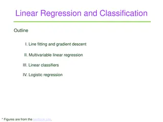
Linear Regression and PCA Analysis
This poster covers the fundamentals and applications of linear regression and principal component analysis (PCA). It explains the concepts, mathematical models, and practical implications of these techniques in data analysis and machine learning. Detailed figures and illustrations are provided to aid in understanding the processes involved in both linear regression and PCA.

Download Presentation

Please find below an Image/Link to download the presentation.
The content on the website is provided AS IS for your information and personal use only. It may not be sold, licensed, or shared on other websites without obtaining consent from the author.If you encounter any issues during the download, it is possible that the publisher has removed the file from their server.
You are allowed to download the files provided on this website for personal or commercial use, subject to the condition that they are used lawfully. All files are the property of their respective owners.
The content on the website is provided AS IS for your information and personal use only. It may not be sold, licensed, or shared on other websites without obtaining consent from the author.
E N D
Presentation Transcript
Poster Title Authors Affiliations Introduction Results Conclusions Include lots of figures and detailed figure captions. Bullet points are much better than long paragraphs. You can easily resize the columns if (for example) a wider middle column better accommodates your figures. You do not need to use the headings in this sample. If you are working in a group: Teach us one thing. Both names should be listed as authors. However, You can do that using your data (ie from written project) or if you have a good artificial data example, you can use that. You should each turn in a different poster as you will be giving different presentations Posters can be related, but there should be an important difference. For example, you may each cover a different technique. Bullet point is too small
Linear regression = Least squares line (single variable x) (or hyperplane for multiple variables) LABELED DATA 2 ??? = ?? ? ?? Supervised learning Data: xi = input data with no noise yi = labels Find function f: R R f(x) = mx + b x = independent variable y = dependent variable (x, y) (x, y ) https://en.wikipedia.org/wiki/Linear_regression
PCA: perturb all variables (x, y) (x, y) UNLABELED DATA Not the least squares line. 1st PCA component = direction of most variance direction = eigenvector with largest eigenvalue. 2nd PCA = direction of 2nd most variance, perpendicular to first. direction = eigenvector with 2nd largest eigenvalue. Modified from https://en.wikipedia.org/wiki/Linear_regression
Example: Principal component analysis (PCA) xi zi = linear combination of xi http://en.wikipedia.org/wiki/File:GaussianScatterPCA.png
https://www.coursera.org/learn/pca-machine-learning/home/info
Same variance in x and y direction, but different co-variances n = ? ( )( ) X X Y Y 1 i i ?? ?2 Var ? = ? 1 = 1 i cov( , ) X Y ) 1 ?=1 ( n https://www.coursera.org/learn/pca-machine-learning/home/info
Now consider two dimensions X=Temperature X=Temperature Y=Humidity Y=Humidity Covariance: measures the correlation between X and Y cov(X,Y)=0: independent Cov(X,Y)>0: move same dir Cov(X,Y)<0: move oppo dir 40 90 40 90 40 90 30 90 15 70 15 70 15 70 30 90 n = 15 70 ( )( ) X X Y Y i i 30 70 = 1 i cov( , ) X Y ) 1 ( n 30 70 30 90 40 70 7 www.cse.buffalo.edu/faculty/azhang/data-mining/pca.ppt 30 90
n = ( )( ) X X Y Y i i = 1 i cov( , ) X Y ) 1 ( n ? 1 ?? ?2 Var ? = ? 1 ?=1 https://www.coursera.org/learn/pca-machine-learning/home/info
for 4 data points for 2 data points for 2 data points https://www.coursera.org/learn/pca-machine-learning/home/info
9 data points n = ( )( ) X X Y Y i i = 1 i cov( , ) X Y ) 1 ( n ? Var ? =1 ?? ?2 ? ?=1 https://www.coursera.org/learn/pca-machine-learning/home/info
More than two attributes: covariance matrix Contains covariance values between all possible dimensions (=attributes): nxn dxd d = dimension = # of attributes or features. = = ( | cov( , )) C c c Dim Dim ij ij i j Example for three attributes (x,y,z): cov( , ) cov( , ) cov( , ) x x x y x z = cov( , ) cov( , ) cov( , ) C y x y y y z cov( , ) cov( , ) cov( , ) z x z y z z 12 www.cse.buffalo.edu/faculty/azhang/data-mining/pca.ppt
9 data points = (0.963855, 0.0361446) n = ( )( ) X X Y Y i i = 1 i cov( , ) X Y ) 1 ( n https://www.coursera.org/learn/pca-machine-learning/home/info
9 data points Equal aspect ratio in python: https://matplotlib.org/stable/gallery/subplots_axes_and_ figures/axis_equal_demo.html = (0.963855, 0.0361446) https://www.coursera.org/learn/pca-machine-learning/home/info
9 data points = (0.963855, 0.0361446) https://www.coursera.org/learn/pca-machine-learning/home/info
Eigenvalues Calculate eigenvalues and eigenvectors x for covariance matrix: Eigenvalues j are used for calculation of [% of total variance] (Vj) for each component j: n = x j = = 100 V n j x n = x 1 x 1 16 www.cse.buffalo.edu/faculty/azhang/data-mining/pca.ppt
for 2 data points https://www.coursera.org/learn/pca-machine-learning/home/info
Principal components 1. principal component (PC1) The eigenvalue with the largest absolute value will indicate that the data have the largest variance along its eigenvector, the direction along which there is greatest variation 2. principal component (PC2) the direction with maximum variation left in data, orthogonal to the 1. PC In general, only few directions manage to capture most of the variability in the data. 18 www.cse.buffalo.edu/faculty/azhang/data-mining/pca.ppt
Eigenvalues Calculate eigenvalues and eigenvectors x for covariance matrix: Eigenvalues j are used for calculation of [% of total variance] (Vj) for each component j: n = x j = = 100 V n j x n = x 1 x 1 19 www.cse.buffalo.edu/faculty/azhang/data-mining/pca.ppt
Principal components - Variance 25 20 Variance (%) 15 10 5 0 PC1 PC2 PC3 PC4 PC5 PC6 PC7 PC8 PC9 PC10 20 www.cse.buffalo.edu/faculty/azhang/data-mining/pca.ppt
A more challenging example data from research on habitat definition in the endangered Baw Baw frog 16 environmental and structural variables measured at each of 124 sites correlation matrix used because variables have different units Philoria frosti http://www.csce.uark.edu/~xintaowu/5073/PCA1.ppt
Eigenvalues % of Variance Cumulative % of Variance Axis Eigenvalue 1 5.855 36.60 36.60 2 3.420 21.38 57.97 3 1.122 7.01 64.98 4 1.116 6.97 71.95 5 0.982 6.14 78.09 6 0.725 4.53 82.62 7 0.563 3.52 86.14 8 0.529 3.31 89.45 9 0.476 2.98 92.42 10 0.375 2.35 94.77 http://www.csce.uark.edu/~xintaowu/5073/PCA1.ppt
Interpreting Eigenvectors correlations between variables and the principal axes are known as loadings each element of the eigenvectors represents the contribution of a given variable to a component 1 2 3 Altitude pH Cond TempSurf Relief maxERht avERht %ER %VEG %LIT %LOG %W H1Moss DistSWH DistSW DistMF 0.3842 -0.1159 -0.2729 0.0538 -0.0765 0.0248 0.0599 0.0789 0.3305 -0.3053 -0.3144 -0.0886 0.1364 -0.3787 -0.3494 0.3899 0.0659 0.1696 -0.1200 -0.2800 0.3855 0.4879 0.4568 0.4223 -0.2087 0.1226 0.0402 -0.0654 -0.1262 0.0101 -0.1283 0.0586 -0.1177 -0.5578 0.3636 0.2621 -0.1462 0.2426 0.2497 0.2278 -0.0276 0.1145 -0.1067 -0.1171 0.4761 0.0042 0.1166 -0.0175 http://www.csce.uark.edu/~xintaowu/5073/PCA1.ppt
Steps of PCA Let be the mean vector (taking the mean of all rows) Adjust the original data by the mean X = X Compute the covariance matrix C of adjusted X Find the eigenvectors and eigenvalues of C. X For matrix C, vectors e (=column vector) having same direction as Ce : eigenvectors of C is e such that Ce= e, is called an eigenvalue of C. Ce= e (C- I)e=0 X Most data mining packages do this for you. 24 www.cse.buffalo.edu/faculty/azhang/data-mining/pca.ppt
Translate data so mean is at the origin. Let v be a unit vector https://ekamperi.github.io/mathematics/2020/11/01/principal-component-analysis-lagrange-multiplier.html
By taking the transpose of the first equation since C is symmetric. https://ekamperi.github.io/mathematics/2020/11/01/principal-component-analysis-lagrange-multiplier.html
Example: Principle component analysis (PCA) xi zi = linear combination of xi http://en.wikipedia.org/wiki/File:GaussianScatterPCA.png
www.stat.columbia.edu/~fwood/Teaching/w4315/Fall2009/pca.pdf

")
 →(x’, y’)")
")


")