Kalman Filter Overview by Po-Chen Wu
Explore the Introduction to Kalman Filter by Po-Chen Wu, covering conceptual overviews, theory, examples, and the need for Kalman Filters in various systems. Understand the optimal estimation process and recursive data processing algorithms used in generating desired quantity estimates. Delve into the problem of estimating optimal system states from measurements and learn about practical applications through theoretical and example-based approaches.

Download Presentation

Please find below an Image/Link to download the presentation.
The content on the website is provided AS IS for your information and personal use only. It may not be sold, licensed, or shared on other websites without obtaining consent from the author. If you encounter any issues during the download, it is possible that the publisher has removed the file from their server.
You are allowed to download the files provided on this website for personal or commercial use, subject to the condition that they are used lawfully. All files are the property of their respective owners.
The content on the website is provided AS IS for your information and personal use only. It may not be sold, licensed, or shared on other websites without obtaining consent from the author.
E N D
Presentation Transcript
Introduction to Kalman Filter Po-Chen Wu Media IC and System Lab Graduate Institute of Electronics Engineering National Taiwan University
Outline Introduction to Kalman Filter Conceptual Overview The Theory of Kalman Filter Simple Example Extended Kalman Filter Po-Chen Wu ( ) Media IC & System Lab 2
Takeaways What is a Kalman Filter? Why do we need Kalman Filters? Po-Chen Wu ( ) Media IC & System Lab 3
Outline Introduction to Kalman Filter Conceptual Overview The Theory of Kalman Filter Simple Example Extended Kalman Filter Po-Chen Wu ( ) Media IC & System Lab 4
Introduction Recursive data processing algorithm Generates optimal estimate of desired quantities given the set of measurements Optimal: For linear system and white Gaussian errors, Kalman filter is best estimate based on all previous measurements. Recursive: doesn t need to store all previous measurements and reprocess all data each time step. Po-Chen Wu ( ) Media IC & System Lab 5
The Problem Black Box System Error Sources External Controls System System State (desired but not known) Optimal Estimate of System State Observed Measurements Measuring Devices Estimator Measurement Error Sources System state cannot be measured directly. Need to estimate optimally from measurements. Po-Chen Wu ( ) Media IC & System Lab 6
Outline Introduction to Kalman Filter Conceptual Overview The Theory of Kalman Filter Simple Example Extended Kalman Filter Po-Chen Wu ( ) Media IC & System Lab 7
Conceptual Overview (1/9) x Lost on the 1-dimensional line Position x(t) Assume Gaussian distributed measurements Po-Chen Wu ( ) Media IC & System Lab 8
Conceptual Overview (2/9) 0.16 0.14 0.12 0.1 0.08 0.06 0.04 0.02 0 0 10 20 30 40 50 60 70 80 90 100 Sextant Measurement at ?1: Mean = ?1and Variance = z1 Optimal estimate of position is: x(t1) = z1 Variance of error in estimate: x Boat in same position at time t2 - Predicted position is z1 2(t1) = z1 2 Po-Chen Wu ( ) Media IC & System Lab 9
Conceptual Overview (3/9) 0.16 0.14 measurement z(t2) 0.12 prediction x (t2) 0.1 0.08 0.06 0.04 0.02 0 0 10 20 30 40 50 60 70 80 90 100 So we have the prediction y (t2) GPS Measurement at t2: Mean = z2and Variance = z2 Need to correct the prediction due to measurement to get x(t2) Closer to more trusted measurement linear interpolation? Po-Chen Wu ( ) Media IC & System Lab 10
Conceptual Overview (4/9) 0.16 corrected optimal estimate x(t2) 0.14 measurement z(t2) 0.12 prediction x (t2) 0.1 0.08 0.06 0.04 0.02 0 0 10 20 30 40 50 60 70 80 90 100 Corrected mean is the new optimal estimate of position New variance is smaller than either of the previous two variances Po-Chen Wu ( ) Media IC & System Lab 11
Conceptual Overview (5/9) Lessons so far: Make prediction based on previous data: x , Take measurement: zk, z Optimal estimate ( y) = Prediction + (Kalman Gain) * (Measurement - Prediction) Variance of estimate = Variance of prediction * (1 Kalman Gain) Po-Chen Wu ( ) Media IC & System Lab 12
Conceptual Overview (6/9) 0.16 x(t2) 0.14 Na ve Prediction x (t3) 0.12 0.1 0.08 0.06 0.04 0.02 0 0 10 20 30 40 50 60 70 80 90 100 At time t3, boat moves with velocity dx dt= u Na ve approach: Shift probability to the right to predict This would work if we knew the velocity exactly (perfect model) Po-Chen Wu ( ) Media IC & System Lab 13
Conceptual Overview (7/9) 0.16 x(t2) 0.14 Na ve Prediction x (t3) 0.12 0.1 0.08 Prediction x (t3) 0.06 0.04 0.02 0 0 10 20 30 40 50 60 70 80 90 100 Better to assume imperfect model by adding Gaussian noise dx dt= u + w Distribution for prediction moves and spreads out Po-Chen Wu ( ) Media IC & System Lab 14
Conceptual Overview (8/9) 0.16 Corrected optimal estimate x(t3) 0.14 Measurement z(t3) 0.12 0.1 0.08 Prediction x (t3) 0.06 0.04 0.02 0 0 10 20 30 40 50 60 70 80 90 100 Now we take a measurement at t3 Need to once again correct the prediction Same as before Po-Chen Wu ( ) Media IC & System Lab 15
Conceptual Overview (9/9) Lessons learnt from conceptual overview: Initial conditions ( xk 1and k 1) Prediction ( xk Use initial conditions and model (eg. constant velocity) to make prediction Measurement (zk) Take measurement Correction ( xk, k) Use measurement to correct prediction by blending prediction and residual always a case of merging only two Gaussians Optimal estimate with smaller variance , k ) Po-Chen Wu ( ) Media IC & System Lab 16
Outline Introduction to Kalman Filter Conceptual Overview The Theory of Kalman Filter Simple Example Extended Kalman Filter Po-Chen Wu ( ) Media IC & System Lab 17
Theoretical Basis Process to be estimated: xk= Axk 1+ Buk+ wk Process Noise (w) with covariance Q Measurement Noise (v) with covariance R zk= Hxk+ vk Kalman Filter Predicted: xk = A xk 1+ Buk is estimate based on measurements at previous time-steps Predicted (a priori) state estimate xk Predicted (a priori) estimate covariance = APk 1AT+ Q Pk Corrected: xk has additional information the measurement at time k + K(zk H xk ) xk= xk HT(HPk HT+ R) 1 K = Pk Pk= (1 KH)Pk Optimal Kalman gain 18
Blending Factor If we are sure about measurements: Measurement error covariance (R) decreases to zero K increases and weights residual more heavily than prediction If we are sure about prediction Prediction error covariance Pk K decreases and weights prediction more heavily than residual decreases to zero Po-Chen Wu ( ) Media IC & System Lab 19
Theoretical Basis Initial estimates for xk 1 and Pk 1 Correction (Measurement Update) Prediction (Time Update) (1) Compute the Kalman Gain HT(HPk HT+ R) 1 (1) Project the state ahead K = Pk = A xk 1+ Buk xk (2) Update estimate with measurement zk + K(zk H xk ) (2) Project the error covariance ahead xk= xk = APk 1AT+ Q (3) Update Error Covariance Pk Pk= (1 KH)Pk Po-Chen Wu ( ) Media IC & System Lab 20
Outline Introduction to Kalman Filter Conceptual Overview The Theory of Kalman Filter Simple Example Extended Kalman Filter Po-Chen Wu ( ) Media IC & System Lab 21
Simple Example (1/4) x Consider a truck on perfectly frictionless, infinitely long straight roads. Initially the truck is stationary at position 0, but it is buffeted this way and that by random acceleration. We measure the position of the truck every t seconds, but these measurements are imprecise; we want to maintain a model of where the truck is and what its velocity is. We show here how we derive the model from which we create our Kalman filter. Po-Chen Wu ( ) Media IC & System Lab 22
Simple Example (2/4) The position and velocity of the truck are described by the linear state space: ??= ? ? We assume that between the (k 1) and k timestep the truck undergoes a constant acceleration of akthat is normally distributed, with mean 0 and standard deviation a. ??= ??? 1+ ?? ??~? 0,? ??= ??? 1+ ??? ? =1 0 t4 4 t3 2 t3 2 t2 2 t t 1, ? = ? = ??T?? 2= t2 Po-Chen Wu ( ) Media IC & System Lab 23
Simple Example (3/4) At each time step, a noisy measurement of the true position of the truck is made. Let us suppose the measurement noise ??is also normally distributed, with mean 0 and standard deviation z. ??= ???+ ?? ??~? 0,? ? = ??2 ? = ? ? Po-Chen Wu ( ) Media IC & System Lab 24
Simple Example (4/4) We know the initial starting state of the truck with perfect precision, so we initialize ?0=0 0 And to tell the filter that we know the exact position, we give it a zero covariance matrix: ?0=0 0 0 0 ( ?0=? 0 ? ) 0 If the initial position and velocity are not known perfectly the covariance matrix should be initialized with a suitably large number, say L, on its diagonal. Po-Chen Wu ( ) Media IC & System Lab 25
Outline Introduction to Kalman Filter Conceptual Overview The Theory of Kalman Filter Simple Example Extended Kalman Filter Po-Chen Wu ( ) Media IC & System Lab 26
Extended Kalman Filter The basic Kalman filter is limited to a linear assumption. The extended Kalman filter (EKF) is the nonlinear version of the Kalman filter which linearizes about an estimate of the current mean and covariance. xk= Axk 1+ Buk+ wk xk= ?(xk 1+ uk) + wk zk= (xk) + vk zk= Hxk+ vk Po-Chen Wu ( ) Media IC & System Lab 27
Theoretical Basis Initial estimates for xk 1 and Pk 1 Correction (Measurement Update) Prediction (Time Update) (1) Compute the Kalman Gain Hk T(HkPk Hk T+ R) 1 (1) Project the state ahead K = Pk = ?( xk 1+ uk) xk (2) Update estimate with measurement zk + K(zk ( xk )) (2) Project the error covariance ahead xk= xk = AkPk 1Ak T+ Q (3) Update Error Covariance Pk Pk= (1 KHk)Pk ? ?x xk ?? ?x xk 1,uk Hk= Ak= Po-Chen Wu ( ) Media IC & System Lab 28
Reference Bishop, Gary, and Greg Welch. "An introduction to the Kalman filter." Proc of SIGGRAPH, Course 8.27599- 23175 (2001): 41. Michael Williams. "Introduction to Kalman Filters." Powerpoint Slides, 5 June 2003 Po-Chen Wu ( ) Media IC & System Lab 29


")
")
")
")
")
")
")
")
")


")
")
")
")