Introduction to R Programming: Statistical & Graphical Methods

R is a programming language developed in 1993 by Ross Ihaka and Robert Gentleman. It offers a wide range of statistical and graphical methods, making it a powerful tool for data analysis and visualization.

• R programming
• Statistical methods
• Graphical analysis
• Data visualization
• Programming language

gracea Follow

Uploaded on Sep 21, 2024 | 0 Views

Download Presentation

Please find below an Image/Link to download the presentation.

The content on the website is provided AS IS for your information and personal use only. It may not be sold, licensed, or shared on other websites without obtaining consent from the author. Download presentation by click this link. If you encounter any issues during the download, it is possible that the publisher has removed the file from their server.

Presentation Transcript

1. Unit IV R programming Prepared By: Bhavana Hotchandani, DCS, INDUS University 1

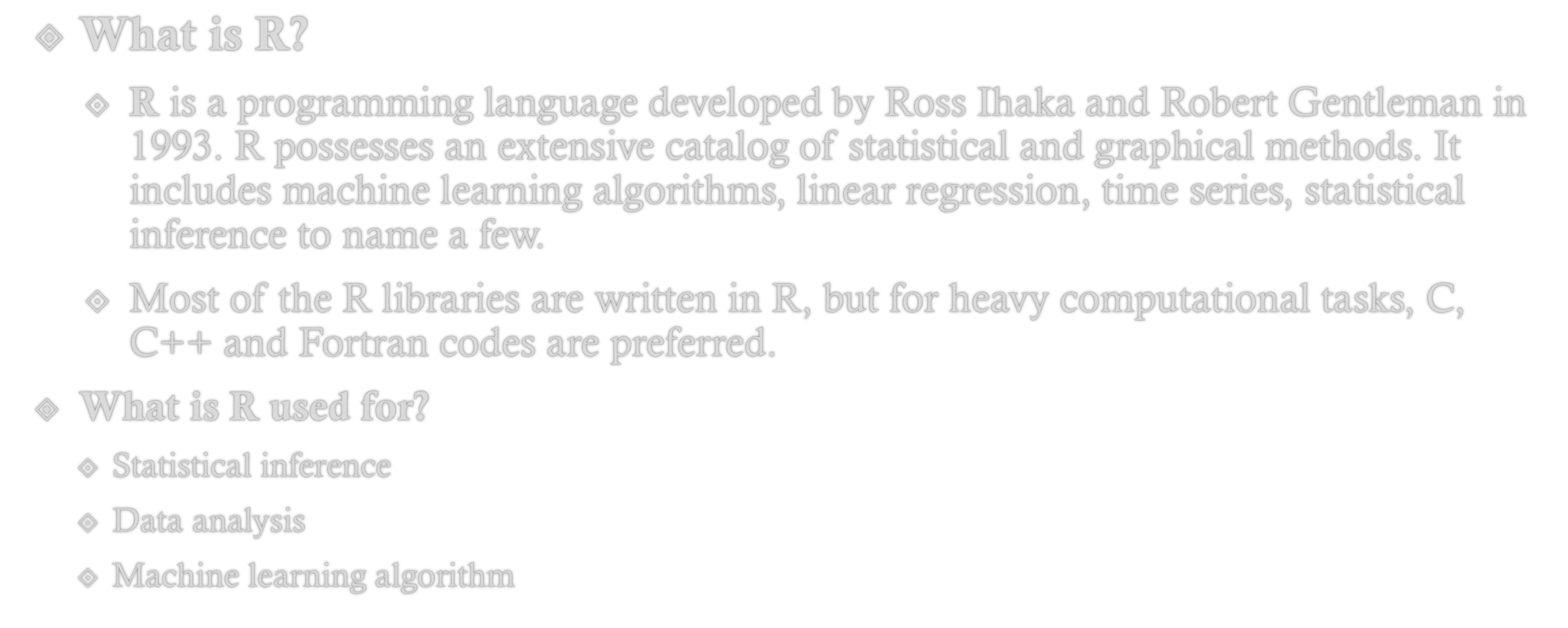
2. R Programming(Introduction & Basics) What is R? R is a programming language developed by Ross Ihaka and Robert Gentleman in 1993. R possesses an extensive catalog of statistical and graphical methods. It includes machine learning algorithms, linear regression, time series, statistical inference to name a few. Most of the R libraries are written in R, but for heavy computational tasks, C, C++ and Fortran codes are preferred. What is R used for? Statistical inference Data analysis Machine learning algorithm 2 Prepared By: Bhavana Hotchandani, DCS, INDUS University

3. Download & Install R is a programming language. To use R, we need to install an Integrated Development Environment (IDE). Rstudio is the Best IDE available as it is user-friendly, open-source and is part of the Anaconda platform. 3 Prepared By: Bhavana Hotchandani, DCS, INDUS University

4. R Data Types, Arithmetic & Logical Operators Basic data types: R Programming works with numerous data types, including Scalars Vectors (numerical, character, logical) Matrices Data frames Lists Basics types 4.5 is a decimal value called numerics. 4 is a natural value called integers. Integers are also numerics. TRUE or FALSE is a Boolean value called logical. The value inside " " or ' ' are text (string). They are called characters. 4 Prepared By: Bhavana Hotchandani, DCS, INDUS University

5. We can check the type of a variable with the class function x <- 28 class(x) y <- "R is Fantastic" class(y) z <- TRUE class(z) 5 Prepared By: Bhavana Hotchandani, DCS, INDUS University

6. Variables Variables store values and are an important component in programming, especially for a data scientist. A variable can store a number, an object, a statistical result, vector, dataset, a model prediction basically anything R outputs. We can use that variable later simply by calling the name of the variable. To declare a variable, we need to assign a variable name. The name should not have space. We can use _ to connect to words. To add a value to the variable, use <- or =. x <- 42 y <- 10 x-y 6 Prepared By: Bhavana Hotchandani, DCS, INDUS University

7. Vectors A vector is a one-dimensional array. We can create a vector with all the basic data type we learnt before. # Numerical vec_num <- c(1, 10, 49) vec_num # Character vec_chr <- c("a", "b", "c") vec_chr # Boolean vec_bool <- c(TRUE, FALSE, TRUE) vec_bool 7 Prepared By: Bhavana Hotchandani, DCS, INDUS University

8. Sum of vector: # Create the vectors vect_1 <- c(1, 3, 5) vect_2 <- c(2, 4, 6) # Take the sum of A_vector and B_vector sum_vect <- vect_1 + vect_2 # Print out total_vector sum_vect Slice a vector slice_vector <- c(1,2,3,4,5,6,7,8,9,10) slice_vector[1:5] 8 Prepared By: Bhavana Hotchandani, DCS, INDUS University

9. Arithmetic Operators +,-,*,/,% or ** Logical Operators The logical statements in R are wrapped inside the []. We can add many conditional statements as we like but we need to include them in a parenthesis. # Create a vector from 1 to 10 logical_vector <- c(1:10) logical_vector>5 FALSE FALSE FALSE FALSE FALSE TRUE TRUE TRUE TRUE TRUE R reads each value and compares it to the statement logical_vector>5. If the value is strictly superior to five, then the condition is TRUE, otherwise FALSE. R returns a vector of TRUE and FALSE. logical_vector[(logical_vector>5)] logical_vector[(logical_vector>4) & (logical_vector<7)] Prepared By: Bhavana Hotchandani, DCS, INDUS University 9

10. What is a Matrix? A matrix is a 2-dimensional array that has m number of rows and n number of columns. In other words, matrix is a combination of two or more vectors with the same data type. Note: It is possible to create more than two dimensions arrays with R. matrix(data, nrow, ncol, byrow = FALSE) data: The collection of elements that R will arrange into the rows and columns of the matrix \ nrow: Number of rows ncol: Number of columns byrow: The rows are filled from the left to the right. We use `byrow = FALSE` (default values), if we want the matrix to be filled by the columns i.e. the values are filled top to bottom. matrix_a <-matrix(1:10, byrow = TRUE, nrow = 5) matrix_a matrix_b <-matrix(1:10, nrow = 5) matrix_b dim(matrix_a) 10 Prepared By: Bhavana Hotchandani, DCS, INDUS University

11. matrix_c <-matrix(1:12, byrow = FALSE, ncol = 3) matrix_c Add a Column to a Matrix with the cbind() # concatenate c(1:5) to the matrix_a matrix_a1 <- cbind(matrix_a, c(1:5)) # Check the dimension dim(matrix_a1) The number of rows of matrices should be equal for cbind work cbind()concatenate columns, rbind() appends rows. 11 Prepared By: Bhavana Hotchandani, DCS, INDUS University

12. Slice a Matrix matrix_c[1,2] selects the element at the first row and second column. matrix_c[1:3,2:3] results in a matrix with the data on the rows 1, 2, 3 and columns 2, 3, matrix_c[,1] selects all elements of the first column. matrix_c[1,] selects all elements of the first row. 12 Prepared By: Bhavana Hotchandani, DCS, INDUS University

13. What is Factor in R? Factors are variables in R which take on a limited number of different values; such variables are often referred to as categorical variables. In a dataset, we can distinguish two types of variables: categorical and continuous. In a categorical variable, the value is limited and usually based on a particular finite group. For example, a categorical variable can be countries, year, gender, occupation. A continuous variable, however, can take any values, from integer to decimal. For example, we can have the revenue, price of a share, etc.. R stores categorical variables into a factor. Let's check the code below to convert a character variable into a factor variable. Characters are not supported in machine learning algorithm, and the only way is to convert a string to an integer. 13 Prepared By: Bhavana Hotchandani, DCS, INDUS University

14. factor(x = character(), levels, labels = levels, ordered = is.ordered(x)) Arguments: x: A vector of data. Need to be a string or integer, not decimal. Levels: A vector of possible values taken by x. This argument is optional. The default value is the unique list of items of the vector x. Labels: Add a label to the x data. For example, 1 can take the label `male` while 0, the label `female`. ordered: Determine if the levels should be ordered. day_vector <- c('evening', 'morning', 'afternoon', 'midday', 'midnight', 'evening') # Convert `day_vector` to a factor with ordered level factor_day <- factor(day_vector, order = TRUE, levels =c('morning', 'midday', 'afternoon', 'evening', 'midnight')) # Print the new variable factor_day 14 Prepared By: Bhavana Hotchandani, DCS, INDUS University

15. What is a Data Frame? A data frame is a list of vectors which are of equal length. A matrix contains only one type of data, while a data frame accepts different data types (numeric, character, factor, etc.). We can create a data frame by passing the variable a,b,c,d into the data.frame() function. We can name the columns with name() and simply specify the name of the variables. data.frame(df, stringsAsFactors = TRUE) df: It can be a matrix to convert as a data frame or a collection of variables to join stringsAsFactors: Convert string to factor by default We can create our first data set by combining four variables of same length. # Create a, b, c, d variables a <- c(10,20,30,40) b <- c('book', 'pen', 'textbook', 'pencil_case') c <- c(TRUE,FALSE,TRUE,FALSE) d <- c(2.5, 8, 10, 7) # Join the variables to create a data frame df <- data.frame(a,b,c,d) df 15 Prepared By: Bhavana Hotchandani, DCS, INDUS University

16. We can see the column headers have the same name as the variables. We can change the column name with the function names(). Check the example below: # Name the data frame names(df) <- c('ID', 'items', 'store', 'price') Df # Print the structure str(df) 16 Prepared By: Bhavana Hotchandani, DCS, INDUS University

17. Slice Data Frame We select the rows and columns to return into bracket precede by the name of the data frame. A data frame is composed of rows and columns, df[A, B]. A represents the rows and B the columns. We can slice either by specifying the rows and/or columns. 17 Prepared By: Bhavana Hotchandani, DCS, INDUS University

18. Append a Column to Data Frame You need to use the symbol $ to append a new variable. # Create a new vector quantity <- c(10, 35, 40, 5) # Add `quantity` to the `df` data frame df$quantity <- quantity df The number of elements in the vector has to be equal to the no of elements in data frame. 18 Prepared By: Bhavana Hotchandani, DCS, INDUS University

19. Select a Column of a Data Frame Sometimes, we need to store a column of a data frame for future use or perform operation on a column. We can use the $ sign to select the column from a data frame. # Select the column ID df$ID Subset a Data Frame In the previous section, we selected an entire column without condition. It is possible to subset based on whether or not a certain condition was true. We use the subset() function. # Select price above 5 subset(df, subset = price > 5) 19 Prepared By: Bhavana Hotchandani, DCS, INDUS University

20. Lists A list is a great tool to store many kinds of object in the order expected. We can include matrices, vectors data frames or lists. A list is collection of objects and we can use them when we need them. We can use list() function to create a list. list(element_1, ...) # Vector with numeric from 1 up to 5 vect <- 1:5 # A 2x 5 matrix mat <- matrix(1:9, ncol = 5) dim(mat) # select the 10th row of the built-in R data set EuStockMarkets df <- EuStockMarkets[1:10,] # Construct list with these vec, mat, and df: my_list <- list(vect, mat, df) my_list 20 Prepared By: Bhavana Hotchandani, DCS, INDUS University

21. Select Elements from List We need to use the [[index]] to select an element in a list. The value inside the double square bracket represents the position of the item in a list we want to extract. my_list[[2]] 21 Prepared By: Bhavana Hotchandani, DCS, INDUS University

22. Built-in Functions Almost everything in R is done through functions. Here I'm only refering to numeric that are commonly used in creating or recoding variables. Function abs(x) sqrt(x) ceiling(x) floor(x) trunc(x) round(x, digits=n) round(3.475, digits=2) is 3.48 signif(x, digits=n) signif(3.475, digits=2) is 3.5 Description absolute value square root ceiling(3.475) is 4 floor(3.475) is 3 trunc(5.99) is 5 22 Prepared By: Bhavana Hotchandani, DCS, INDUS University

23. Function Description mean(x, trim=0, na.rm=FALSE) mean of object x # trimmed mean, removing any missing values and # 5 percent of highest and lowest scores mx <- mean(x,trim=.05,na.rm=TRUE) standard deviation of object(x). also look at var(x) for variance and mad(x) for median absolute deviation. median sd(x) median(x) quantile(x, probs) quantiles where x is the numeric vector whose quantiles are desired and probs is a numeric vector with probabilities in [0,1]. # 30th and 84th percentiles of x y <- quantile(x, c(.3,.84)) range range(x) sum(x) Sum diff(x, lag=1) lagged differences, with lag indicating which lag to use min(x) minimum max(x) maximum scale(x, center=TRUE, scale=TRUE) column center or standardize a matrix. 23 Prepared By: Bhavana Hotchandani, DCS, INDUS University

24. Conditions & Loops R has the standard control structures you would expect. expr can be multiple (compound) statements by enclosing them in braces { }. It is more efficient to use built-in functions rather than control structures whenever possible. If-else if (cond) expr if (cond) expr1 else expr2 for for (var in seq) expr while while (cond) expr switch switch(expr, ...) 24 Prepared By: Bhavana Hotchandani, DCS, INDUS University

25. User-written Functions One of the great strengths of R is the user's ability to add functions. In fact, many of the functions in R are actually functions of functions. The structure of a function is given below. myfunction <- function(arg1, arg2, ... ){ statements return(object) } Invoking a function y <- myfunction(x) 25 Prepared By: Bhavana Hotchandani, DCS, INDUS University

26. Reading csv and xlsx Read CSV One of the most widely data store is the .csv (comma-separated values) file formats. R loads an array of libraries during the start-up, including the utils package. This package is convenient to open csv files combined with the reading.csv() function. Here is the syntax for read.csv read.csv(file, header = TRUE, sep = ",") Argument: file: PATH where the file is stored header: confirm if the file has a header or not, by default, the header is set to TRUE sep: the symbol used to split the variable. By default, `,`. The PATH needs to be a string value. We should always specify the extension of the file name. 26 Prepared By: Bhavana Hotchandani, DCS, INDUS University

27. df <- read.csv(file = 'mtcars.csv',header = TRUE, sep = ',') head(df) length(df) class(df$model) R, by default, returns character values as Factor. We can turn off this setting by adding stringsAsFactors = FALSE. 27 Prepared By: Bhavana Hotchandani, DCS, INDUS University

28. Read Excel files Excel files are very popular among data analysts. Spreadsheets are easy to work with and flexible. R is equipped with a library readxl to import Excel spreadsheet. read_excel() read_excel(PATH, sheet = NULL, range= NULL, col_names = TRUE) arguments: -PATH: Path where the excel is located -sheet: Select the sheet to import. By default, all -range: Select the range to import. By default, all non-null cells -col_names: Select the columns to import. By default, all non-null columns 28 Prepared By: Bhavana Hotchandani, DCS, INDUS University

29. We can control what cells to read in 2 ways Use n_max argument to return n rows Use range argument combined with cell_rows or cell_cols For example, we set n_max equals to 5 to import the first five rows. df <-read_excel("cancer_data1.xlsx", n_max =5, col_names =TRUE) df If we change col_names to FALSE, R creates the headers automatically. 29 Prepared By: Bhavana Hotchandani, DCS, INDUS University

30. Linear Regression Regression analysis is one of the most important fields in statistics and machine learning. There are many regression methods available. Linear regression is one of them. What Is Regression? Regression searches for relationships among variables. For example, you can observe several employees of some company and try to understand how their salaries depend on the features, such as experience, level of education, role, city they work in, and so on. This is a regression problem where data related to each employee represent one observation. The presumption is that the experience, education, role, and city are the independent features, while the salary depends on them. Similarly, you can try to establish a mathematical dependence of the prices of houses on their areas, numbers of bedrooms, distances to the city center, and so on. 30 Prepared By: Bhavana Hotchandani, DCS, INDUS University

31. Generally, in regression analysis, you usually consider some phenomenon of interest and have a number of observations. Each observation has two or more features. Following the assumption that (at least) one of the features depends on the others, you try to establish a relation among them. It is used to show the linear relationship between a dependent variable and one or more independent variables. In other words, you need to find a function that maps some features or variables to others sufficiently well. The dependent features are called the dependent variables, outputs, or responses. The independent features are called the independent variables, inputs, or predictors. Regression problems usually have one continuous and unbounded dependent variable. The inputs, however, can be continuous, discrete, or even categorical data such as gender, nationality, brand, and so on. It is a common practice to denote the outputs with ? and inputs with ?. 31 Prepared By: Bhavana Hotchandani, DCS, INDUS University

32. Where is Linear Regression Used? Evaluating Trends and Sales Estimates Analyzing the Impact of Price Changes Assessing Risk Linear relationship basically means that when one (or more) independent variables increases (or decreases), the dependent variable increases (or decreases) too: For linear functions, we have this formula: y = a*x + b https://data36.com/linear-regression-in-python-numpy-polyfit/ 32 Prepared By: Bhavana Hotchandani, DCS, INDUS University

33. When Do You Need Regression? Typically, you need regression to answer whether and how some phenomenon influences the other or how several variables are related. For example, you can use it to determine if and to what extent the experience or gender impact salaries. Regression is also useful when you want to forecast a response using a new set of predictors. For example, you could try to predict electricity consumption of a household for the next hour given the outdoor temperature, time of day, and number of residents in that household. Regression is used in many different fields: economy, computer science, social sciences, and so on. Its importance rises every day with the availability of large amounts of data and increased awareness of the practical value of data. Linear regression is probably one of the most important and widely used regression techniques. It s among the simplest regression methods. One of its main advantages is the ease of interpreting results. 33 Prepared By: Bhavana Hotchandani, DCS, INDUS University

34. Example with Python import numpy as np import matplotlib.pyplot as plt import pandas as pd from sklearn.linear_model import LinearRegression data = pd.read_csv('LRdata.csv') X = data.iloc[:, 0].values.reshape(-1, 1) # values converts it into a numpy array Y = data.iloc[:, 1].values.reshape(-1, 1) # -1 means that calculate the dimension of rows, but have 1 column linear_regressor = LinearRegression() linear_regressor.fit(X, Y) Y_pred = linear_regressor.predict(X) plt.scatter(X, Y) plt.plot(X, Y_pred, color='red') plt.show() plt.savefig('graph.png') 34 Prepared By: Bhavana Hotchandani, DCS, INDUS University

35. Good Links Data Wrangling and Manipulation https://towardsdatascience.com/data-wrangling-with-pandas-5b0be151df4e https://www.pluralsight.com/guides/data-wrangling-pandas https://medium.com/analytics-vidhya/python-data-manipulation-fb86d0cdd028 https://data-flair.training/blogs/data-wrangling-with-python/ https://elitedatascience.com/python-data-wrangling-tutorial https://www.earthdatascience.org/courses/earth-analytics-bootcamp/data-wrangling/data- wrangling-pandas/ https://www.statmethods.net/management/sorting.html https://www.guru99.com/r-import-data.html https://swcarpentry.github.io/r-novice-inflammation/11-supp-read-write-csv/ 35 Prepared By: Bhavana Hotchandani, DCS, INDUS University