Decision Trees in Machine Learning
Decision trees are a popular machine learning technique that maps attribute values to decisions. They involve tests that lead from the root to leaf nodes, with each internal node representing a test on an attribute. The use cases range from the restaurant waiting problem to boolean classification and shape recognition. Decision trees offer simplicity, efficiency, and easy-to-understand results, making them valuable tools in data analysis and pattern recognition.

Download Presentation

Please find below an Image/Link to download the presentation.
The content on the website is provided AS IS for your information and personal use only. It may not be sold, licensed, or shared on other websites without obtaining consent from the author.If you encounter any issues during the download, it is possible that the publisher has removed the file from their server.
You are allowed to download the files provided on this website for personal or commercial use, subject to the condition that they are used lawfully. All files are the property of their respective owners.
The content on the website is provided AS IS for your information and personal use only. It may not be sold, licensed, or shared on other websites without obtaining consent from the author.
E N D
Presentation Transcript
Decision Trees Outline I. Decision trees II. Learning decision trees from examples III. Entropy and attribute choice ** Figures are from the textbook site (or by the instructor).
Restaurant Waiting Problem Decide whether to wait for a table at a restaurant. Output: a Boolean variable WillWait (true where we do wait for a table). Input: a vector of ten attributes, each with discrete values: 1. Alternate: whether there is a suitable alternative restaurant nearby. 2. Bar: whether the restaurant has a comfortable bar area to wait in. 3. Fri/Sat: true on Fridays and Saturdays. 4. Hungry: whether we are hungry right now. 5. Patrons: how many people are in the restaurant (values: None, Some, and Full). 6. Price: the restaurant s price range ($, $$, $$$). 7. Raining: whether it is raining outside. 8. Reservation: whether we made a reservation. 9. Type: the kind of restaurant (French, Italian, Thai, or burger). 10. WaitEstimate: host s wait estimate: 0-10, 10-30, 30-60, or >60 minutes. 26 32 42= 9,216 possible combinations of attribute values.
Training Examples The correct output is given for only 12 out of 9,216 examples. We need to make our best guess at the missing 9,204 output values.
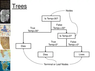
I. What is a Decision Tree? A decision tree maps a set of attribute values to a decision . It performs a sequence of tests, starting at the root and descending down to a leaf (which specifies the output value). Each internal node corresponds to a test of the value of an attribute. A decision tree for the restaurant waiting problem ?1
Boolean Classification Inputs are discrete values. Outputs are either true (a positive example) or false (a negative one). Positive examples: Patrons = Some Patrons = Full WaitEstimate = 0 10 Patrons = Full WaitEstimate = 10 30 Hungry = Yes Alternate = No Negative examples: Patrons = No Patrons = Full WaitEstimate > 60
Shape Recognition Tree A robotic hand can recognize curved shapes from differential invariants (expressions of curvature, torsion, etc.) constructed over tactile data. // Values of ??1 and ??2 do not vary // at different contour points (i.e., they are // invariants on the shape)? https://faculty.sites.iastate.edu/jia/files/inline-files/IJRR05.pdf
Why Decision Trees? They yield nice, concise, and understandable results. They represent simple rules for classifying instances that are described by discrete attribute values. Decision tree learning algorithms are relatively efficient linear in the size of the decision tree and the size of the data set. Decision trees are often among the first to be tried on a new data set. They are not good with real-valued attributes.
Expressiveness of a Decision Tree Equivalent logical statement of a decision tree: Output Path1 Path2 (one statement for Output = Yes and another for Output = No) Disjunctive normal form (DNF) where Path?= (??1= ??1 ??2= ??2 ) Path1 Path? attribute value yes yes yes Any sentence in propositional logic can be converted into a DNF. Any sentence in propositional logic can expressed as a decision tree.
II. Learning DTs from Examples Problem Find a tree that is a) consistent with the training examples (in, e.g, restaurant waiting) and b) as small as possible. Generally, it s intractable to find a smallest consistent tree. A suboptimaltree can be constructed with some simple heuristics. Greedy divide-and-conquer strategy: Test the most important attribute first. make the most difference to the classification Recursively solve the smaller subproblems.
Poor and Good Attributes Poor attribute Type: four outcomes each with the same number of positive as negative examples Good attributes Patrons and Hungry: effective separations of positive and negative examples
Four Cases 1. All positive (or all negative) remaining examples. Done. 2. Mixed positive and negative remaining examples. Choose the best attribute to split them. 3. No examples left. ??? Return the most common output value (e.g., ) for the example set used in constructing the parent (???) ?1 ?2 ?3 Yes 4. No attributes left but both positive and negative examples. Return the most common output value of these examples (by a majority vote) No
Algorithm for Learning DTs // case 3 // case 1 // case 4 // case 2
Output Decision Tree Considerably simpler! ?2 Original decision tree ?1
Learning Curve happy graph 100 randomly generated examples in the restaurant domain. Split them randomly into a training set and a test set. Split 20 times for each size (1 99) of the training set. Average the results of the 20 trials.
III. Entropy and Attribute Choice Importance of an attribute is measured using the notion of information gain defined in terms of entropy. measure of the uncertainty of a random variable: the more information, the less entropy. A fair coin has 1 bit of entropy as it is equally likely to come up heads and tails when flipped. A four-sided die has 2 bits of entropy since there are 22 equally likely choices. An unfair coin that comes up heads 99% of the time would have an entropy measure that is close to zero.
Entropy Random variable ? with values ?? having probability ? ??. Entropy of ?: ? log2? 1 ? ? = ?(??)log2 ?(??) ? = ?(??)log2?(??) ? Entropy measures the expected amount of information conveyed by identifying the outcome of a random trial.
Entropy Examples A fair coin ? Fair = 0.5log20.5 + 0.5log20.5 = 1 (bit) There is maximum surprise in this case. A coin with known outcome (e.g., head) ? Head = 1 log21 = 0 (bit) There is no uncertainty at all no information. A loaded coin with 99% heads ? Loaded = 0.99log20.99 + 0.01log20.01 0.08 (bits) A four-sided die ? Die4 = 4 0.25log20.25 = 2 (bits)
Entropy of a Boolean Variable A Boolean random variable that is true with probability ?. ? ? = ?(1 ?) ? ? = (?log2? + (1 ?)log2(1 ?)) ? Loaded = ?(0.99) 0.08 A training set contains ? positive examples and ? negative examples. ? ? Output = ? ? + ? ? = ? = 6 ? 0.5 = 1
Choice of an Attribute An attribute ? has ? distinct values. ? divides the training set ? into subsets ?1, ,??. Each subset ?? has ?? positive examples and ?? negative examples. ? ? and ? = ?? ? = ?? ?=1 ?=1 ?? This implies an additional ? ??+?? bits of information. Consider a randomly chosen example from the training set. Its attribute ? value is in ?? with probability ??+ ??/ ? + ? . Expected entropy remaining after testing attribute ? is ??+?? ?+?? ?? ? Remainder ? = ?=1 ??+??
Information Gain Expected reduction in entropy from the attribute test on ?: ? Gain ? = ? Remainder ? ? + ? ? ? ??+ ?? ? + ? ?? = ? ? ? + ? ??+ ?? ?=1 Choose the attribute ? among the remaining attributes to maximize Gain ? .
Information Gain ? ? ??+ ?? ? + ? ?? Gain ? = ? ? ? + ? ??+ ?? ?=1 1 2 2 12? 1 2+ 2 12? 1 2+ 4 12? 2 4+ 4 12? 2 4 = 0 bits Gain Type = ? 1 2 2 12? 0 2+ 4 12? 4 4+ 6 12? 2 6 0.541 bits Gain Patrons = ?