Computer Graphics Rendering Pipeline Overview
Introduction to the forward rendering pipeline in computer graphics, covering clipping, culling, transformations, primitive assembly, rasterization, and fragment processing. Details on viewport transformations, vertex processing, and visible primitives are included. Clipping techniques for points, lines, and polygons are discussed along with the importance of clipping in the clip space post-projection transformation.
Download Presentation

Please find below an Image/Link to download the presentation.
The content on the website is provided AS IS for your information and personal use only. It may not be sold, licensed, or shared on other websites without obtaining consent from the author.If you encounter any issues during the download, it is possible that the publisher has removed the file from their server.
You are allowed to download the files provided on this website for personal or commercial use, subject to the condition that they are used lawfully. All files are the property of their respective owners.
The content on the website is provided AS IS for your information and personal use only. It may not be sold, licensed, or shared on other websites without obtaining consent from the author.
E N D
Presentation Transcript
CENG 477 Introduction to Computer Graphics Forward Rendering Pipeline Clipping and Culling
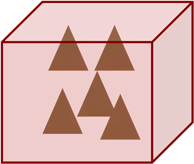
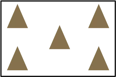
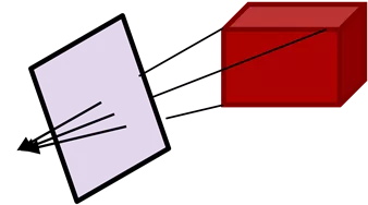
Rendering Pipeline Sequence of operations that is used to draw primitives defined in a 3D coordinate system on a 2D window Can be implemented on hardware or software Two notable APIs: OpenGL and D3D Not static: Constantly evolving to meet the demands of the industry Rendering Pipeline 2D Window 3D World
Rendering Pipeline Overview Pixels Vertices 1. Get vertices in specific order and connectivity information Process vertices Create primitives from connected vertices Clip and cull primitives to eliminate invisible ones Transform primitives to screen space (preserve z) Rasterize primitives to obtain fragments Process fragments to obtain visible pixels with color Vertex Processing Fragment Processing 2. 3. Transformed vertices Fragments 4. Primitive Assembly 5. Rasterization Primitives 6. Primitives with 2D coordinates and z Clipping and Culling 7. Viewport Transform Visible primitives
Until Now Pixels Vertices We ve done transformations: model to world to camera to clip space We skip over primitive assembly as it is mostly straightforward We ll look at clipping and culling today We ve done viewport transformations Yet to come rasterization: lines, triangles, interpolation Yet to come fragment processing (blending, depth testing, alpha testing, etc) afterwards Vertex Processing Fragment Processing Transformed vertices Fragments Primitive Assembly Rasterization Primitives Primitives with 2D coordinates and z Clipping and Culling Viewport Transform Visible primitives
Clipping In modern graphics API, there are essentially three kinds of primitives: points, lines, and triangles Point clipping: straightforward Reject a point if its coordinates are outside the viewing volume Line clipping Cohen-Sutherland algorithm Liang-Barsky algorithm Polygon clipping Sutherland-Hodgeman algorithm
Clipping Clipping is done in the clip space which is a result of applying projection (orthographic or perspective) transformation After perspective transformation the w component of a point becomes equal to z 2? ? ? ? + ? ? ? ? + ? ? ? ? + ? ? ? 1 0 0 2? 0 0 ????= ? ? 2?? ? ? 0 0 0 0 0
Clipping To find the actual point in the canonical viewing volume, we divide by this last component However, clipping is performed before dividing by w (that is z) for two reasons: w may be equal to 0 in which case division would be undefined ? ? 1 we can directly compare ? ? ? thus avoiding an extra division The same goes for y and z components Instead of comparing 1
Clipping For simplicity, however, in the following we assume that clipping is performed against a 2D box with coordinates between [xmin, xmax] and [ymin, ymax] The same ideas can be easily generalized to 3D
Line Clipping Cohen-Sutherland Alg. Handle trivial accept and trivial rejects first For non-trivial cases, subdivide lines until all parts can be trivially accepted and rejected Trivial accept/reject lines Non-trivial cases
Line Clipping Cohen-Sutherland Alg. Assign region codes to the end points of lines: Bit0 = 1 if region is to the left of left edge, 0 otherwise Bit1 = 1 if region is to the right of right edge, 0 otherwise Bit2 = 1 if region is below the bottom edge, 0 otherwise Bit3 = 1 if region is above the top edge, 0 otherwise 1001 1000 1010 How many bits would we need? How many regions would we have in 3D? 0001 0000 0010 0100 0110 0101
Line Clipping Cohen-Sutherland Alg. Assign the codes to the end points of the line: cv0 = 0001 cv1 = 1010 v1 1001 1000 1010 0001 0000 0010 v0 0100 0110 0101 If both codes are zero, the line can be trivially accepted If bitwise and of region codes is not zero, then the line can be trivially rejected
Line Clipping Cohen-Sutherland Alg. Non-trivial cases: Iteratively subdivide into two segments such that one or both segments can be discarded, until we can trivially reject or accept it Intersection of the outpoint and extended viewport border is computed (i.e. with the parametric equation for the line) and this new point replaces the outpoint v1 v1 1001 1000 1010 1001 1000 1010 0001 0000 0010 0001 0000 0010 v0 v0 0100 0110 0100 0110 0101 0101
Line Clipping Cohen-Sutherland Alg. Non-trivial cases: Iteratively subdivide into two segments such that one or both segments can be discarded, until we can trivially reject or accept it Intersection of the outpoint and extended viewport border is computed (i.e. with the parametric equation for the line) and this new point replaces the outpoint v1 v1 1001 1000 1010 1001 1000 1010 v'1 0001 0000 0010 0001 0000 0010 v'0 v'0 no trivial rejection 0100 0110 0100 0110 0101 0101
Line Clipping Cohen-Sutherland Alg. Advantages: If the chances of trivial accept/reject are high, this is a very fast algorithm This can happen if the clipping rectangle is very large or very small Disadvantages: Non-trivial lines can take several iterations to clip Because testing and clipping are done in a fixed order, the algorithm will sometimes perform needless clipping
Line Clipping Liang-Barsky Algorithm Uses the idea of parametric lines Classifies lines as potentially entering and potentially leaving to speed up computation (approximately 40% speed-up over Cohen-Sutherland Alg.) Line equation: p = v0 + (v1-v0)t ymax tl tl t of interest? te te ymin xmin xmax
Line Clipping Liang-Barsky Algorithm Uses the idea of parametric lines Classifies lines as potentially entering and potentially leaving to speed up computation (approximately 40% speed-up over Cohen-Sutherland Alg.) Line equation: p = v0 + (v1-v0)t ymax tl tl t of interest LARGEST te SMALLEST tl te te ymin xmin xmax
Line Clipping Liang-Barsky Algorithm Uses the idea of parametric lines Classifies lines as potentially entering and potentially leaving to speed up computation (approximately 40% speed-up over Cohen-Sutherland Alg.) Line equation: p = v0 + (v1-v0)t reject if _______? ymin xmin xmax
Line Clipping Liang-Barsky Algorithm Uses the idea of parametric lines Classifies lines as potentially entering and potentially leaving to speed up computation (approximately 40% speed-up over Cohen-Sutherland Alg.) Line equation: p = v0 + (v1-v0)t te tl reject if te > tl ymin xmin xmax
Line Clipping Liang-Barsky Algorithm Uses the idea of parametric lines Classifies lines as potentially entering and potentially leaving to speed up computation (approximately 40% speed-up over Cohen-Sutherland Alg.) v1 = (x1, y1) ymax Goal: Given the line v0, v1 determine: - The part of the line is inside the viewing rectangle. p = (x, y) v0 = (x0, y0) Note: p = v0 + (v1-v0)t ymin xmin xmax
Line Clipping Liang-Barsky Algorithm Potentially entering (PE) and leaving (PV): Why do we say potentially? v0,v1 is potentially entering the left edge as x1 x0 > 0 v2,v3 is potentially leaving the left edge as x3 x2 < 0 v3 v7 v1 v5 The situation is reversed for the right edge: v2 v0 v6 v4 v4,v5 is potentially leaving the right edge as x5 x4 > 0 v6,v7 is potentially entering the right edge as x7 x6 < 0 Right Left
Line Clipping Liang-Barsky Algorithm Similar for bottom and top edges: v0,v1 is potentially entering the bottom edge as y1 y0 > 0 v2,v3 is potentially leaving the bottom edge as y3 y2 < 0 v6 Top v5 The situation is reversed for the top edge: v7 v4 v2 v1 v4,v5 is potentially leaving the top edge as y5 y4 > 0 v6,v7 is potentially entering the top edge as y7 y6 < 0 Bottom v3 v0
Line Clipping Liang-Barsky Algorithm Observation: If a line is first leaving then entering, it cannot be visible v1 PE v1 PE PL PL v0 v0 v1 v1 PE PE PL PL v0 v0
Line Clipping Liang-Barsky Algorithm Visible lines are first entering then leaving: v1 PL v1 PL PE PE v0 v0 v1 v1 PL PL PE PE v0 v0
Line Clipping Liang-Barsky Algorithm Mathematical interpretation: if (tPL < tPE): visible = false; Note: p = v0 + (v1-v0)t So at intersection points, we need to compute the t value as well as whether the line is PE or PL at that point. v1 PE v1 PE v1 PL v1 PL PL PL PE PE v0 v0 v0 v0 v1 v1 PL v1 PL v1 PE PE PE PE PL PL v0 v0 v0 v0
Line Clipping Liang-Barsky Algorithm Computing t value at every edge: xleft = x0 + (x1-x0)t t = (xleft x0) / (x1 x0) xright = x0 + (x1-x0)t t = (xright x0) / (x1 x0) ybottom = y0 + (y1-y0)t t = (ybottom y0) / (y1 y0) ytop = y0 + (y1-y0)t t = (ytop y0) / (y1 y0) But this does not help us to know if line is entering or leaving at that point. Solution: look at the sign of dx, dy: v0,v1 is potentially entering the left edge if dx = (x1 x0) > 0 v0,v1 is potentially entering the right edge if dx = (x1 x0) < 0 or dx > 0 v0,v1 is potentially entering the bottom edge if dy = (y1 y0) > 0 v0,v1 is potentially entering the top edge if dy = (y1 y0) < 0 or dy > 0
Line Clipping Liang-Barsky Algorithm Finding intersection type: Entering left edge if dx > 0. Entering right edge if -dx > 0. Entering bottom edge if dy > 0. Entering top edge if -dy > 0. Finding t: For left edge: t = (xleft x0) / (x1 x0) = (xleft x0) / dx For right edge: t = (xright x0) / (x1 x0) = (xright x0) / dx = (x0 xright) / (-dx) For bottom edge: t = (ybottom y0) / (y1 y0) = (yleft y0) / dy For top edge: t = (ytop y0) / (y1 y0) = (ytop y0) / dy = (y0 ytop) / (- dy)
Line Clipping Liang-Barsky Algorithm For lines parallel to edges: v1 = (x1, y1) if dx == 0 and xmin x0 > 0: // left reject; else if dx == 0 and x0 - xmax > 0: // right reject; else if dy == 0 and ymin y0 > 0: // bottom reject; else if dy == 0 and y0 - ymax > 0: // top reject; ymax v0 = (x0, y0) ymin xmin xmax
Line Clipping Liang-Barsky Algorithm Putting it all together: tE = 0; tL = 1; visible = false; if visible(dx, xmin x0. tE, tL): // left if visible (-dx, x0 xmax . tE, tL): // right if visible (dy, ymin y0 . tE, tL): // bottom if visible (-dy, y0 ymax . tE, tL): // top visible = true; if (tL < 1): x1 = x0 + dxtL; y1 = y0 + dytL; if (tE > 0): x0 = x0 + dxtE; y1 = y0 + dytE; bool visible(den, num, tE, tL): if (den > 0): // potentially entering t = num / den; if (t > tL): return false; if (t > tE) tE = t; elseif (den < 0): // potentially leaving t = num / den; if (t < tE): return false; if (t < tL) tL = t; else if num > 0: // line parallel to edge return false; return true;
Example Left Edge v1 v1 v0 v0 PE with small positive t (tE = t) Right Edge v1 PL with large positive t (tL = t) v0
Example Bottom Edge v1 v1 v0 v0 PE with negative t (tE not updated) Top Edge PL with t > 1 (tL not updated) v1 v0
Example Result v1 Smallest tL v0 Largest tE
Polygon Clipping Sutherland Hodgeman Algorithm Difficult problem as we need to deal with many cases:
Polygon Clipping Sutherland Hodgeman Algorithm Divide and conquer approach makes it manageable: Solve a series of simple and identical problems. When combined, the overall problem is solved. Here, the simple problem is to clip a polygon against a single clip edge: Clip against right edge
Polygon Clipping Sutherland Hodgeman Algorithm Clip against bottom edge Clip against left edge
Polygon Clipping Sutherland Hodgeman Algorithm Clip against top edge
Polygon Clipping Sutherland Hodgeman Algorithm This is accomplished by visiting the input vertices from v0 to vN and then back to v0 for each clip boundary. At every step we add 0, 1, or 2 vertices to the output: Inside Outside Inside Outside Inside Outside Inside Outside vi vi vi+1 vi vi+1 vi v'i+1 v'i+1 vi+1 vi+1 Add vi+1 to output Add v i+1 to output Add nothing to output Add v i+1 and vi+1to output
Polygon Clipping Sutherland Hodgeman Algorithm Inside Outside n a What is v i+1? vi+1 vi v'i+1 Add v i+1 to output
Polygon Clipping Sutherland Hodgeman Algorithm Inside Outside n a What is p = v i+1? Call v = vi and w = vi+1 p = v + t(w-v) Denote d1 = n.(v-a) and d2 = n.(w-a) vi+1 vi v'i+1 Add v i+1 to output p - a = (v-a) + t(w-a (v-a)) //subtract a n.(p - a) = n.(v-a) + t(n(w-a) n(v-a)) //multiply by n 0 = d1 + t(d2 d1) t = d1 / (d1 d2) What if v is on the plane? What if w is on the plane? Also, d1 is + (-), d2 is - (+)
Polygon Clipping In Action Maintain In and Out list, which will help you extract result IN OUT p1 p2
Polygon Clipping In Action Maintain In and Out list, which will help you extract result IN OUT p1 p2 p2 p2
Polygon Clipping In Action Maintain In and Out list, which will help you extract result IN OUT p1 p2 p2 p2 p3 p4
Polygon Clipping In Action Maintain In and Out list, which will help you extract result IN OUT p1 p2 p2 p4 p5 p2 p3 p4 p4
Culling Complex scenes contains many objects. Objects closer to the camera occlude objects further away. Rendering time can be saved if these invisible objects are culled (i.e. eliminated, discarded, thrown away). Three common culling strategies are: View volume (frustum) culling Backface culling Occlusion culling
View Volume (Frustum) Culling The removal of geometry outside the viewing volume. No OpenGL support: it is the programmer s responsibility to cull what is outside. From lighthouse3d.com
View Volume (Frustum) Culling First determine the equations of the planes that make up the boundary of the view volume (6 planes): Plane equation: (p a).n = 0 Here, a is a point on the plane and n is the normal. Plug the vertices of each primitive for p. If we get: (p a).n > 0 for any plane, the vertex is outside. If all vertices are outside, then the primitive is outside and can be culled. Using a bounding box or bounding sphere for complex models is a better solution.
Backface Culling For closed polygon models, back facing polygons are guaranteed to be occluded by front facing polygons (so they don t need to be rendered) OpenGL supports backface culling: glCullFace(GL_BACK) and glEnable(GL_CULL_FACE). From http://wwwisg.cs.uni-magdeburg.de/~oscar
Backface Culling For closed polygon models, back facing polygons are guaranteed to be occluded by front facing polygons (so they don t need to be rendered) OpenGL supports backface culling: glCullFace(GL_BACK) and glEnable(GL_CULL_FACE). Without BFC With BFC
Backface Culling For closed polygon models, back facing polygons are guaranteed to be occluded by front facing polygons (so they don t need to be rendered) Also useful in hidden line removal Wireframe Hidden lines removed
Backface Culling Polygons whose normals face away from the eye are called back facing polygons. v2 w v0 w n v v eye eye n v v v1 v1 v0 v2 Front facing triangle n.v < 0 Back facing triangle n.v > 0
Backface Culling Note the v is the vector from the eye to any point on the polygon (you can take the polygon center). You cannot use the view vector! w From http://omega.di.unipi.it
