Centrality Measures in Social Network Analysis

Discover the importance of centrality in social network analysis through measures like Degree Centrality, Eigenvector Centrality, and Katz Centrality. Learn how these metrics identify the most central vertices in a network based on factors such as connections, citations, and influence. Explore the concepts, calculations, and applications of centrality in analyzing network structures.

Download Presentation

Please find below an Image/Link to download the presentation.
The content on the website is provided AS IS for your information and personal use only. It may not be sold, licensed, or shared on other websites without obtaining consent from the author.If you encounter any issues during the download, it is possible that the publisher has removed the file from their server.
You are allowed to download the files provided on this website for personal or commercial use, subject to the condition that they are used lawfully. All files are the property of their respective owners.
The content on the website is provided AS IS for your information and personal use only. It may not be sold, licensed, or shared on other websites without obtaining consent from the author.
E N D
Presentation Transcript
Centrality Social network analysis Which are the most important or central vertices in a network? Degree centrality: the degree of a vertex Citation network: the number of citations of a paper is simply its in- degree.
Eigenvector Centrality Not all neighbors are equivalent. A vertex s importance is increased by having connections to other vertices that are themselves important. The idea is to define the centrality of a vertex as the sum of the centralities of its neighbors. Suppose we guess initially vertex i has centrality xi(0) Then a better one is
Eigenvector Centrality Write x(0) as a linear combination of the eigenvectors vi of the adjacency matrix A The limiting centrality should be proportional to the leading eigenvector v1.
Definition Bonacich (1987) Let k1be the leading eigenvalue of A. The centralities of all the vertices satisfy Eigenvector centralities are nonnegative (easy to see from the limit of the multiplication of A and an initial nonnegative guess x(0)). Normalization problem (require the sum to be a constant)
Eigenvector centrality for directed networks Can be extended to directed networks (e.g., web pages). The problem of zero centrality in a directed network A has centrality 0 as there are no incoming edges (seems reasonable for a web page) But B has one incoming edge from A. The centrality of B is still 0 because A has centrality 0. The centralities are all 0 in an acyclic network.
Katz centrality Give every vertex a small amount of centrality for free. are positive constants. In matrix terms, where 1 is the vector (1,1, ,1)T. Katz centrality: set =1
Choosing the constant k1is the largest eigenvalue of A Then This is because v1(the eigenvector of A corresponding to k1) is an eigenvector of with eigenvalue 0. The range Computing the Katz centrality by iterating is better than inverting the matrix directly.
PageRank Trademark of Google A variation of Katz centrality Divided by the out-degree The problem of a vertex with zero out-degree Easy fix: since a vertex with zero out-degree contribute zero to the centralities of other vertices. We may simply set
PageRank In matrix terms, D is a diagonal matrix with Google uses =1 and =0.85 (no theory behind this choice). Need to make sure that the value of should be less than the inverse of the largest eigenvalue of AD-1. Special case when =0 and =1. PageRank reduces to the degree centrality.
Web surfing Initially, every web page is chosen randomly with the same probability. With probability , perform a random walk on the web by randomly choosing a hyperlink in a page. With probability 1- , stop the random walk and restart the web surfing. PageRank is simply the steady state probability that a web page is visited by this web surfing. Phase type distribution of a random variable
Web surfing Let =1- . PTis the transition probability matrix a Markov chain. The steady state probability vector can be computed via
Hubs and authorities Every vertex has two types of centralities: hub centrality and authority centrality. Authorities: vertices that contain useful (or important) information (e.g., an important scientific paper) Hubs: vertices that tells where the best authorities are (e.g. a good review paper) Hyperlink-induced topic search (HITS) first proposed by Kleinberg 1999 in J. ACM
Hubs and authorities The authority centrality of a vertex (denoted by xi) is defined to be proportional to the sum of the hub centralities of the vertices (denoted by yj) that point to it: The hub centrality of a vertex is defined to be proportional to the sum of the authorities centralities of the vertices it points to:
Hubs and authorities In matrix terms, Note that both AATand ATA have the same eigenvalues. AAT is the cocitation matrix and the authority centrality is the eigenvector centrality of the cocitation network. ATA is bibliographic coupling matrix and the hub authority is the eigenvector centrality of the bibliographic coupling network.
Closeness centrality Measure the mean distance from a vertex to other vertices. dijis the length of a geodesic path from vertex i to vertex j. The mean geodesic distance from vertex i to other vertices When j=i, dii=0. It is better to use
Closeness centrality The mean geodesic distance gives low values for more central verticies. Closeness centrality Ci: Problems: The values are too closely spaced. Movie database: Christopher Lee 2.4138, Donald Pleasense 2.4164. If the network is disconnected, then the closeness centralities are all 0. If we only average over vertices in a component, then it favors small components.
Harmonic mean closeness centrality This solves the problem of disconnected networks. It also gives more weights to vertices that are close to vertex i than to those far away. Can be used for the study of small world effect by defining the harmonic mean distance
Betweenness centrality Measure the extent to which a vertex lies on paths between other vertices. Let be 1 if vertex i lies on the geodesic path from s to t. The betweenness centrality xiis given by Vertices with high betweenness centrality may have considerable influence within a network by virtue of their control of information passing between others.
Modification The problem with more than one geodesic paths between s and t. Let gstbe the number of geodesic paths between s and t. The (modified) betweenness measure of vertex i is
Broker in social networks Vertex A lies on a bridge between two groups in a network. Vertex A has high betweenness centrality But it does not have high degree centrality or eigenvector centrality.
Maximum betweenness Maximum betweenness: consider a star graph with n nodes The central vertex has n-1 vertices attached to it. The central vertex is on every geodesic path between two different vertices and the path from the central vertex to itself. The betweenness of the central vertex is n(n-1)+1=n2-n+1.
Minimum betweenness In a connected network, there are n-1 geodesic paths to a particular vertex (and the other way around). Adding the path from the vertex to itself results in the minimum 2(n-1)+1 betweenness centrality. This happens when a vertex is a leaf (an isolated vertex with a single connection to the network) of a network. The ratio of largest and smallest possible betweenness values is
Other betweenness centralities Maximum flow betweenness: is the number of flows through vertex i from s to t. The problem is the way to choose maximum flows is not unique. Random-walk betweenness: is the expected number of visits of vertex i from s to t.