Understanding the Fibonacci Method for Function Optimization
The Fibonacci method offers a systematic approach to finding the minimum of a function even if it's not continuous. By utilizing a sequence of Fibonacci numbers, this method helps in narrowing down the interval of uncertainty to determine the optimal solution through a series of experiments. Despite some limitations, including known initial uncertainty intervals and unimodality assumptions, this method provides a structured process for optimization tasks.

Download Presentation

Please find below an Image/Link to download the presentation.
The content on the website is provided AS IS for your information and personal use only. It may not be sold, licensed, or shared on other websites without obtaining consent from the author. Download presentation by click this link. If you encounter any issues during the download, it is possible that the publisher has removed the file from their server.
E N D
Presentation Transcript
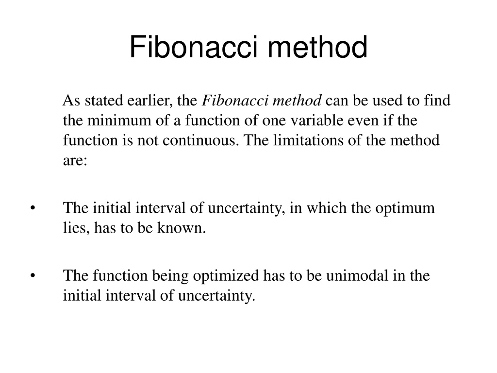
Fibonacci method As stated earlier, the Fibonacci method can be used to find the minimum of a function of one variable even if the function is not continuous. The limitations of the method are: The initial interval of uncertainty, in which the optimum lies, has to be known. The function being optimized has to be unimodal in the initial interval of uncertainty.
Fibonacci method The limitations of the method (cont d): The exact optimum cannot be located in this method. Only an interval known as the final interval of uncertainty will be known. The final interval of uncertainty can be made as small as desired by using more computations. The number of function evaluations to be used in the search or the resolution required has to be specified before hand.
Fibonacci method This method makes use of the sequence of Fibonacci numbers, {Fn}, for placing the experiments. These numbers are defined as: = = 1 + F F 0 1 = = , , 4 , 3 , 2 F F F n 1 2 n n n which yield the sequence 1,1,2,3,5,8,13,21,34,55,89,...
Fibonacci method Procedure: Let L0be the initial interval of uncertainty defined by a x b and n be the total number of experiments to be conducted. Define F L n = n * 2 2 L 0 F and place the first two experiments at points x1and x2, which are located at a distance of L2*from each end of L0.
Fibonacci method Procedure: This gives F = + = + * 2 2 n x a L a L 1 0 F n F F = = = + * 2 2 1 n n x b L b L a L 2 0 0 F F n n Discard part of the interval by using the unimodality assumption. Then there remains a smaller interval of uncertainty L2given by: F F = = = * 2 2 1 n n 1 L L L L L 2 0 0 0 F F n n
Fibonacci method Procedure: The only experiment left in will be at a distance of F F = = * 2 2 2 n n L L L 0 2 F F 1 n n from one end and F F = = * 2 3 3 n n L L L L 2 0 2 F F 1 n n from the other end. Now place the third experiment in the interval L2so that the current two experiments are located at a distance of: F L F n n F = = * 3 3 3 n n L L 0 2 F 1
Fibonacci method Procedure: This process of discarding a certain interval and placing a new experiment in the remaining interval can be continued, so that the location of the jth experiment and the interval of uncertainty at the end of j experiments are, respectively, given by: F n j = * L L 1 j j F ) 2 ( n j F ) 1 ( n j = L L 0 j F n
Fibonacci method Procedure: The ratio of the interval of uncertainty remaining after conducting j of the n predetermined experiments to the initial interval of uncertainty becomes: L F ) 1 ( j n j = L F 0 n and for j = n, we obtain 1 L F = = 1 n L F F 0 n n
Fibonacci method The ratio Ln/L0will permit us to determine n, the required number of experiments, to achieve any desired accuracy in locating the optimum point.Table gives the reduction ratio in the interval of uncertainty obtainable for different number of experiments.
Fibonacci method Position of the final experiment: In this method, the last experiment has to be placed with some care. Equation F L n j = * L 1 j j F ) 2 ( n j gives * n 1 L F = = 0 for all n 2 L F 1 2 n Thus, after conducting n-1 experiments and discarding the appropriate interval in each step, the remaining interval will contain one experiment precisely at its middle point.
Fibonacci method Position of the final experiment: In this method, the last experiment has to be placed with some care. Equation F L n j = * L 1 j j F ) 2 ( n j gives * n 1 L F = = 0 for all n 2 L F 1 2 n Thus, after conducting n-1 experiments and discarding the appropriate interval in each step, the remaining interval will contain one experiment precisely at its middle point.
Fibonacci method Position of the final experiment: However, the final experiment, namely, the nth experiment, is also to be placed at the center of the present interval of uncertainty. That is, the position of the nth experiment will be the same as that of ( n-1)th experiment, and this is true for whatever value we choose for n. Since no new information can be gained by placing the nth experiment exactly at the same location as that of the (n-1)th experiment, we place the nth experiment very close to the remaining valid experiment, as in the case of the dichotomous search method.
Fibonacci method Example: Minimize f(x)=0.65-[0.75/(1+x2)]-0.65 x tan-1(1/x) in the interval [0,3] by the Fibonacci method using n=6. Solution: Here n=6 and L0=3.0, which yield: ) 0 . 3 ( 13 F n 5 F = = 153846 . 1 = L 2 * n L 2 0 Thus, the positions of the first two experiments are given by x1=1.153846 and x2=3.0-1.153846=1.846154 with f1=f(x1)=- 0.207270 and f2=f(x2)=-0.115843. Since f1is less than f2, we can delete the interval [x2,3] by using the unimodality assumption.
Fibonacci method Solution:
Fibonacci method Solution: The third experiment is placed at x3=0+ (x2-x1)=1.846154- 1.153846=0.692308, with the corresponding function value of f3=- 0.291364. Since f1is greater than f3, we can delete the interval [x1,x2]
Fibonacci method Solution: The next experiment is located at x4=0+ (x1-x3)=1.153846- 0.692308=0.461538, with f4=-0.309811. Noting that f4is less than f3, we can delete the interval [x3,x1]
Fibonacci method Solution: The location of the next experiment can be obtained as x5=0+ (x3- x4)=0.692308-0.461538=0.230770, with the corresponding objective function value of f5=-0.263678. Since f4is less than f3, we can delete the interval [0,x5]
Fibonacci method Solution: The final experiment is positioned at x6=x5+ (x3-x4)=0.230770+(0.692308- 0.461538)=0.461540 with f6=-0.309810. (Note that, theoretically, the value of x6should be same as that of x4; however,it is slightly different from x4due to the round off error). Since f6 > f4, we delete the interval [x6, x3] and obtain the final interval of uncertainty as L6= [x5, x6]=[0.230770,0.461540].
Fibonacci method Solution: The ratio of the final to the initial interval of uncertainty is 230770 . 0 . 0 461540 L = = 6 076923 . 0 0 . 3 L 0 This value can be compared with 1 L F = = 1 n L F F 0 n n which states that if n experiments (n=6) are planned, a resolution no finer than 1/Fn= 1/F6=1/13=0.076923 can be expected from the method.