Hypothesis Testing and Statistics in Science
This collection of images and quotes explores the concepts of hypothesis testing, statistics, and the relationship between theory and measurement in science. It delves into the famous quote by Mark Twain about the deceptive nature of figures and provides examples of hypothesis testing problems in research. The importance of considering uncertainties in measurements, as demonstrated by Tycho Brahe, is also highlighted. The content touches upon real-world experiments like the g-2 experiment, showcasing the comparison between experimental results and theoretical predictions.
Download Presentation

Please find below an Image/Link to download the presentation.
The content on the website is provided AS IS for your information and personal use only. It may not be sold, licensed, or shared on other websites without obtaining consent from the author. Download presentation by click this link. If you encounter any issues during the download, it is possible that the publisher has removed the file from their server.
E N D
Presentation Transcript
Statistics and Hypothesis Testing in Science Allen Mincer New York University July 2019 1 BNL June 2019
On Statistics Mark Twain popularized the saying [see end of quote] in Chapters from My Autobiography, published in the North American Review in 1906. "Figures often beguile me," he wrote, "particularly when I have the arranging of them myself; in which case the remark attributed to Disraeli would often apply with justice and force: 'There are three kinds of lies: lies, damned lies, and statistics. https://en.wikipedia.org/wiki/Lies,_damned_lies,_and_statistics (The actual actual of the quote seems to be unknown) 2 BNL June 2019
Introduction to Hypothesis Testing 3 BNL June 2019
Hypothesis Testing Question: A theory predicts a measurement should give 7 Measurement gives 6 What can we say about the theory from the measurement? BNL June 2019
Hypothesis Testing Question: A theory predicts a measurement should give 7 Measurement gives 6 What can we say about the theory from the measurement? Question: A theory predicts a measurement should give 2.00233183714 Measurement gives 2.00233184160 What can we say about the theory from the measurement? BNL June 2019
Hypothesis Testing Problem: A theory predicts a measurement should give 7 Measurement gives 6 What can we say about the theory from the measurement? Problem: A theory predicts a measurement should give 2.00233183714 Measurement gives 2.00233184160 What can we say about the theory from the measurement? Tycho Brahe: In addition to making observations of unprecedented accuracy, Tycho also developed the concept of attaching an uncertainty to each of his measurements http://ircamera.as.arizona.edu/NatSci102/NatSci102/lectures/tycho.htm One cannot really make a statement about agreement or disagreement between measurement and theory or between measurements without knowing the uncertainties.
g-2 The second example above came from the g-2 experiment G.W. Bennett et.al., Phys. Rev. D73, 072003 (2006) Exper. (g-2)/2: 0.00116592080 ( 54 33) = 0.00000000063 Standard Model: 0.00116591857 0.00000000080 (0.00116591820 0.00000000073) Experiment Theory = 0.00000000223 (0.00000000260) BNL June 2019
Quantifying agreement or disagreement We measure some variable X and get the value xM. Assume we understand our measurement and its uncertainties well enough to determine the probability density function (pdf) p(x| ) such that if the true value of X is then the probability of a measurement giving (xM- x/2 < x < xM+ x/2) = p(xM| )dx The probability of any particular value of a continuous variable is zero. So can t say anything about the true value of X from p(xM| ) alone. Instead, we typically determine the probability of a fluctuation at least as big as what we measured. Example: For gaussian distributed uncertainty in measurement, probability of 2 or more above the central value = 2.8% So we can ask, for example, what is the number such that if X= then xM is 2 more than x. The probability of measuring X >=xMif is the true value is then less than 2.8%.
Hypothesis Testing We use this sort of pdf quantification to decide whether theory and experiment agree in a process called hypothesis testing. Define Null and Alternative Hypotheses H0 and H1. eg. Null is existing theory is OK, alternative is the new theory is correct. Unless we can make a measurement which would have a result which is impossible under the existing theory, we must decide using chosen probabilities. Hypothesis test: Make a measurement of some variable X. If the measured value xM lies in some region of values (corresponding to some probability) we will retain H0, otherwise we will reject H0 and accept H1. Error of first kind: Rejecting H0 when it is true. Error of second kind: Accept H0 when it is false. Eg. (Laplace) H0: prisoner is innocent. If evidence exceeds criterion reject H0 and say prisoner is guilty Error of first kind: Find innocent person guilty. Error of second kind: Find guilty person innocent. In any test, must decide what priorities are. In general making one error smaller makes other bigger ( reasonable doubt vs preponderance of evidence )
Selecting critical regions Above ideas used in one guise or another in all hypothesis tests in science. Consider the pdf s sketched below. We will retain the null hypothesis if xM < XT. Otherwise we reject it. As we move the green line to the right, we decrease the error of the first kind (integral of P(x|H0) above the line) and increase error of the second kind (integral of P(x|H1) below the line) Curve need not be normal, but easy to calculate probabilities for normal Where do you put the green line? P(x|H0) P(x|H1) BNL June 2019 XT X
Selecting critical regions Above ideas used in one guise or another in all hypothesis tests in science. Consider the pdf s sketched below. We will retain the null hypothesis if xM < XT. Otherwise we reject it. As we move the green line to the right, we decrease the error of the first kind (integral of P(x|H0) above the line) and increase error of the second kind (integral of P(x|H1) below the line) Curve need not be normal, but easy to calculate probabilities for normal Where do you put the green line? The choice of permissible error is completely arbitrary: there no scientific or mathematical way to favor a particular value of XT. P(x|H0) P(x|H1) BNL June 2019 X XT
But beware of the physical interpretation of the normal distribution Does it make sense to grade a class this way? What is an average student? What are the deviations from average? Pregnancy and the meaning of average woman Does the average human gestation time mean that a woman going longer than average should be induced? How much longer? What if that woman has a history of longer pregnancies? BNL June 2019
Beware a subtle trap P(xM| ) P( |xM) (Is Bayesian statistics a cure?) Example: A medical test gives positive result if someone has a disease 99% of the time, and only 1% false negatives. A person tests positive. What is the probability they have the disease? BNL June 2019
Beware a subtle trap P(xM| ) P( |xM) (Is Bayesian statistics a cure?) Example: A medical test gives positive result if someone has a disease 99% of the time, and only 1% false negatives. A person tests positive. What is the probability they have the disease? Assume that this is a rare disease that only 1/1,000,000 in the population have Assume we test the full population: The one who has it will test positive. 0.01 * 999,999 ~ 10,000 others will test positive So only 1/10,001 = 0.01% of those who test positive have the disease.
p values If we measure xM, the integral of p(x|H0) above xM is called the p value of the measurement. It is the probability that if the null hypothesis were correct we would get a value at least as large as the measured one. A small p value means that it is very unlikely that one would get a measurement this large under H0. P(x|H0) xM X Note that it is statistically dangerous to use the p-value to decide how significant a result is, as opposed to just comparing the result to a threshold determined before looking at the data.
Example 1: Eddington Eclipse Expeditions 16 BNL June 2019
Eddington Eclipse Expeditions 1 Reading: Relativity and Eclipses: The British expeditions of 1919 and their predecessors, J. Earman and C. Glymour, Hist. Stud. Phys. Sci. 11:1 1980 pp. 49 85 Earman and Glymour review results of the 3 measurements overseen by Eddington in 1919 to measure deflection of starlight by the sun as viewed during a solar eclipse Possibilities considered: Light massless, so zero deflection. M= E/c2gives 0.87 General relativity: 1.74 17
Eddington Eclipse Expeditions 2 A. Crommelin and C. Davidson Sobral, N.E. 50 miles inland from the coast of Brazil Sobral 3.43m focal length astrographic telescope 0.86 s.d 0.48 Sobral 19 foot focal length 4 inch aperture unequivocally the best. 1.98 probable error 0.12 s.d. 0.178 A. Eddington and E. Cottingham, Principe, island off the coast of West Africa. Astrographic telescope 1.61 probable error 0.30 s.d. 0.444 J. Earman and C. Glymour: `The evidence that the Sobral 1.98 mean with 0.178 standard deviation provides for the Einstein value of 1.74 is not enormously better than the evidence that the Principe astrographic 1.61 mean and 0.444 standard deviation provides for the Newtonian value of 0.87 . The 1.98 mean is about 1.3 standard deviations away from 1.74 ; the 1.61 mean is about 1.7 standard deviations away from 0.87 18 MEPhi May 2015
Eddington Eclipse Expeditions 3 A. Crommelin and C. Davidson Sobral, N.E. 50 miles inland from the coast of Brazil Sobral 3.43m focal length astrographic telescope 0.86 s.d 0.48 Sobral 19 foot focal length 4 inch aperture unequivocally the best. 1.98 probable error 0.12 s.d. 0.178 A. Eddington and E. Cottingham, Principe, island off the coast of West Africa. Astrographic telescope 1.61 probable error 0.30 s.d. 0.444 J. Earman and C. Glymour: `The evidence that the Sobral 1.98 mean with 0.178 standard deviation provides for the Einstein value of 1.74 is not enormously better than the evidence that the Principe astrographic 1.61 mean and 0.444 standard deviation provides for the Newtonian value of 0.87 . The 1.98 mean is about 1.3 standard deviations away from 1.74 ; the 1.61 mean is about 1.7 standard deviations away from 0.87 But 1.98 with s.d. 0.178 rules out 0.87, but 1.61 s.d 0.444 and 0.86 s.d 0.48 do not rule out 1.74 ! 19 MEPhi May 2015
Example 2: AIDS Vaccine 20 BNL June 2019
AIDS Vaccine 1 Reading: Vaccine for AIDS Passes Trial; Limits of Success to be Studied, D.G. McNeil Jr., NY Times Sep. 25, 2009 p. A1. If AIDS Went the Way of Smallpox, D.G. McNeil Jr., NY Times Sep. 27, 2009, Week In Review, p. 1. Tested RV144, a combination of two genetically engineered vaccines, neither of which had worked on humans before. 6 year clinical trial in which more than 16,402 volunteers (men and women ages 18 30) in Thailand were vaccinated. Cost $105M 74 who got placebos were infected; 51 who got the vaccine were infected. Col. Jerome H. Kim, physician and manager of the Army s HIV vaccine program, said it was statistically significant and meant that the vaccine was 31.2% effective 21 BNL June 2019
AIDS Vaccine 2 74 who got placebos were infected; 51 who got the vaccine were infected. Comment 1: Placebo P = 74 74 = 74 8.6 Vaccinated V = 51 51 = 51 7.1 P V = 74 51 (74+51) = 23 11.2 Is 2 statistically significant? 22 BNL June 2019
AIDS Vaccine 3 74 who got placebos were infected; 51 who got the vaccine were infected. Comment 1: Placebo P = 74 74 = 74 8.6 Vaccinated V = 51 51 = 51 7.1 P V = 74 51 (74+51) = 23 11.2 Is 2 statistically significant? Comment 2: Null hypothesis is it doesn t work The average expected is then (74+51)/2 = 62.5 About 1.5 sigma from 51 and 74 23 BNL June 2019
AIDS Vaccine 4 74 who got placebos were infected; 51 who got the vaccine were infected. Comment 1: Placebo P = 74 74 = 74 8.6 Vaccinated V = 51 51 = 51 7.1 P V = 74 51 (74+51) = 23 11.2 Is 2 statistically significant? Comment 2: Null hypothesis is it doesn t work The average expected is then (74+51)/2 = 62.5 About 1.5 sigma from 51 and 74 Comment 3: What does it mean for a vaccine to be 31.2% effective? (of course too many decimal places in 31.2) Can 2 useless vaccines together make a good one? What is the Bayseian statistics on this? 24 BNL June 2019
Example 3: Choice Rationalization 25 BNL June 2019
Cognitive Dissonance 1 Reading: And Behind Door No. 1, a Fatal Flaw, J. Tierney, NY Times, Science Times, April 8, 2008, p. F1 Choice rationalization: once we reject something, we tell ourselves we never really liked it anyway (and thereby spare ourselves the painfully dissonant thought that we made the wrong choice). 2007 Yale experiment with monkeys: Presented choice of red and blue cadies (M&Ms). If they chose red, they were given a choice of blue and green. 2/3 of the time they choose green Explained as monkeys also show cognitive dissonance 26 BNL June 2019
Cognitive Dissonance 1 Reading: And Behind Door No. 1, a Fatal Flaw, J. Tierney, NY Times, Science Times, April 8, 2008, p. F1 Choice rationalization: once we reject something, we tell ourselves we never really liked it anyway (and thereby spare ourselves the painfully dissonant thought that we made the wrong choice). 2007 Yale experiment with monkeys: Presented choice of red and blue candies (M&Ms). If they chose red, they are given a choice of blue and green. 2/3 of the time they choose green Explained as monkeys also show cognitive dissonance But this is just the Monty Hall problem: 27 BNL June 2019
Monty Hall Problem 1 Behind one of these 3 doors: 1 2 3 28 BNL June 2019
Monty Hall Problem 2 1 2 3 You choose 1 29 BNL June 2019
Monty Hall Problem 3 1 2 3 You chose 1 Monty Hall shows you what is behind 3 30 BNL June 2019
Monty Hall Problem 4 You are given the choice to switch from 1 to 2. Should you switch? 1 2 3 31 BNL June 2019
Monty Hall Problem 5 True door 1st choice Switch Result Don t Switch Result 1 1 Lose Win 2 Win Lose 3 Win Lose So you win 2/3 1/3 Why isn t probability 50-50? Because MH biased it! If MH doesn t show you a bad door, then: True door 1st choice Switch Result Don t Switch Result 1 1 Lose 2/2 Win 2 Win 1/2 Lose 3 Win 1/2 Lose 32 So you win 2/6 = 1/3 1/3
Cognitive Dissonance 2 3 ways to choose red over blue: Result of 2nd choice: 33 Since Monkey chose red at first, twice as many ways to to keep green
Example 4: ESP 34 BNL June 2019
ESP Experiment Reading: R. L. Park, Voodoo Science, Oxford University Press, 2002, pp. 40 to 43 J.B. Rhine Duke University, 1934: Hundreds of thousands of ESP deck (cards with 5 different shapes) trials. Finds success rate slightly higher than 20% Irving Langmuir (1932 Nobel Prize for molecular films studies) asks to visit Rhine. Rhine agrees and even urged Langmuir to publish his views. Says that result would be to attract more graduate students and funding. Result: Langmuir finds Rhine threw out results from people who got very low scores, because they disliked him and were purposely guessing wrong. Reporter didn t understand statistics, and wrote that a famous Nobel laureate was checking into ESP . Rhine was overwhelmed with new graduate students and offers of financial support. BNL June 2019 35
Example 5: Millikan 36 BNL June 2019
Rejection of Data Reading: An Introduction to Error Analysis, J.R. Taylor, University Science Books, 1997 Chapter 6. Millikan s Published and Unpublished Data on Oil Drops, D. Franklin, Historical Studies in the Physical Sciences, 11:2, 185 201 (1981) In Defense of Robert Andrews Millikan, D. Goodstein, Engineering and Science 2000 vol. 4 p.30 My Work with Millikan on the Oildrop Experiment, H. Fletcher, Physics Today June (1982) p. 43 Chauvenet scriterion: If the suspected number of measurements as least as deviant as the suspect measurement is less than one- half, then the suspect measurement should be rejected. Obviously, the choice of one-half is arbitrary, but it is also reasonable and can be defended. 37 BNL June 2019
Millikan Oil Drop Experiment Millikan s Published and Unpublished Data on Oil Drops, D. Franklin, Historical Studies in the Physical Sciences, 11:2, 185 201 (1981) In presenting his final results in 1913, Millikan stated that the 58 drops under discussion had provided his entire set of data. It is to be remarked, too, that this is not a selective set of drops but represents all of the drops experimented upon during 60 consecutive days during which time the apparatus was taken down several times and set up anew. Basic accusation is that Millikan s goal was to show that the uncertainty in his method was smaller than for what other did, so he threw out drops that gave divergent results, and selectively analyzed the drops kept. Indeed, if the thrown out drops are included, the average stays within errors but the spread is smaller. D. Goodstein: Millikan was referring not to the drops kept for e but for for Stokes s Law. Millikan threw out other drops because as an experimenter who knew his apparatus, he knew what to trust. 38 BNL June 2019
Example 6: publication bias and p hacking 39 BNL June 2019
Publication Bias and p hacking Publication Bias: An experiment not showing a new result will rarely be interesting enough to publish. What fraction of experiments conducted wind up finding something new? If the criterion for rejecting the null hypothesis is p<0.1, then 10% of conducted experiments will reject the null hypothesis when if it is correct. p hacking: A single experiment can ask 10 different questions and on average 1 of these will have a p value <0.1 40 BNL June 2019
Disclaimer Please don t confuse this as attacking all the use of statistics in of science. The point here is that it is very easy to get things wrong. So if you read about something that you think makes no sense, you may be right. And avoid believing the result you prefer just because you prefer it. 41 BNL June 2019


