Finite Element Analysis of Heat Transfer Problems
Analogy between stress analysis and heat conduction analysis is discussed. Various thermal problems, including steady-state heat transfer and governing differential equations, are explored. Conservation of energy and boundary conditions are detailed for solving thermal analysis problems.

Download Presentation

Please find below an Image/Link to download the presentation.
The content on the website is provided AS IS for your information and personal use only. It may not be sold, licensed, or shared on other websites without obtaining consent from the author. Download presentation by click this link. If you encounter any issues during the download, it is possible that the publisher has removed the file from their server.
E N D
Presentation Transcript
CHAP 5 FINITE ELEMENTS FOR HEAT TRANSFER PROBLEMS FINITE ELEMENT ANALYSIS AND DESIGN Nam-Ho Kim 1
HEAT CONDUCTION ANALYSIS Analogy between Stress and Heat Conduction Analysis Structural problem Displacement Stress/strain Displacement B.C. Surface traction force Body force Heat transfer problem Temperature (scalar) Heat flux (vector) Fixed temperature B.C. Heat flux B.C. Internal heat generation Thermal conductivity Young s modulus In finite element viewpoint, two problems are identical if a proper interpretation is given. More Complex Problems Coupled structural-thermal problems (thermal strain). Radiation problem 2
THERMAL PROBLEM Goals: = [ ]{ } T { } Q K T Thermal load Nodal temperature Conductivity matrix Solve for temperature distribution for a given thermal load. Boundary Conditions Essential BC: Specified temperature Natural BC: Specified heat flux 3
STEADY-STATE HEAT TRANSFER PROBLEM Fourier Heat Conduction Equation: Heat flow from high temperature to low temperature dT = q kAdx x Thermal conductivity (W/m/ C ) Heat flux (Watts) Examples of 1D heat conduction problems Thigh Tlow Thigh qx qx Tlow 4
GOVERNING DIFFERENTIAL EQUATION Conservation of Energy Energy In + Energy Generated = Energy Out + Energy Increase + = + E E E U in generated out Two modes of heat transfer through the boundary Prescribed surface heat flow Qs per unit area Convective heat transfer h: convection coefficient (W/m2/ C ) ( ) = Q h T T h T Qs dq dx x Qg + D q x x q x A dx 5
GOVERNING DIFFERENTIAL EQUATION cont. Conservation of Energy at Steady State No change in internal energy ( U = 0) dq dx ( ) + + + = + q Q P x h T T P x Q A x q x x x s g x E E gen in E out P: perimeter of the cross-section dq Q A dx ( ) = + + hP T T Q P, 0 x L x g s Apply Fourier Law d dT dx + ( ) + + = kA Q A hP T T Q P 0, 0 x L g s dx Rate of change of heat flux is equal to the sum of heat generated and heat transferred 6
GOVERNING DIFFERENTIAL EQUATION cont. Boundary conditions Temperature at the boundary is prescribed (essential BC) Heat flux is prescribed (natural BC) Example: essential BC at x = 0, and natural BC at x = L: T(0) T dT kA q dx = = 0 = L x L 7
DIRECT METHOD Follow the same procedure with 1D bar element No need to use differential equation Element conduction equation Heat can enter the system only through the nodes Qi: heat enters at node i (Watts) Divide the solid into a number of elements Each element has two nodes and two DOFs (Ti and Tj) For each element, heat entering the element is positive N 2 1 Q1 Q2 QN Q3 j i e ( ) e ( ) e jq iq L(e) Tj Ti xi xj 8
ELEMENT EQUATION Fourier law of heat conduction ( ) T T dT dx j L i = = (e) i q kA kA (e) From the conservation of energy for the element (T T) + = (e) i (e) j j L i = + q q 0 (e) j q kA (e) Combine the two equation = T T (e) i (e) j q q 1 1 kA L i Element conductance matrix (e) 1 1 j Similar to 1D bar element (k = E, T = u, q = f) 9
ASSEMBLY Assembly using heat conservation at nodes Remember that heat flow into the element is positive Equilibrium of heat flow: T T Q Q 1 1 N i = (e) i 2 2 Q q = [ ] K i T ( ) e 1 = N N T Q N N Same assembly procedure with 1D bar elements Applying BC Striking-the-rows works, but not striking-the-columns because prescribed temperatures are not usually zero Q2 3 1 (1) (2) 2q 2q Element 2 Element 1 2 10
EXAMPLE Calculate nodal temperatures of four elements A = 1m2, L = 1m, k = 10W/m/ C Q4 = 200W T1 T2 T3 T4 T5 x 200 C 1 2 3 4 Q2 = 500W Q3 = 0 Q5 = 0 Q1 Element conduction equation T 1 1 10 T 1 1 (1) 1 (1) 2 T T q q (2) 2 (2) 3 1 1 q q 1 = 2 = 10 1 1 2 3 T T T T (4) 4 (4) 5 (3) 3 (3) 4 1 1 1 1 q q q q 4 3 = = 10 10 1 1 1 1 5 4 11
EXAMPLE cont. Assembly Q Q Q Q Q T T T T T (1) 1 + + + 1 1 0 0 0 1 2 1 0 0 0 1 2 1 0 0 0 1 2 1 0 0 0 1 1 q 1 1 (1) 2 (2) 3 (3) 4 (2) 2 (3) 3 (4) 4 q q q q q q 2 2 = = 10 3 3 4 4 (4) 5 q 5 5 Boundary conditions (T1 = 200 oC, Q1 is unknown) 200 T T T T 1 1 0 0 0 0 0 0 Q 500 0 200 0 1 1 2 1 2 = 10 0 0 0 1 2 1 3 0 0 1 2 1 4 0 1 1 5 12
EXAMPLE cont. Boundary conditions Strike the first row 200 T T T T 1 2 0 0 0 0 0 1 0 0 0 500 0 200 0 2 1 2 1 = 10 3 1 2 1 4 0 1 1 5 Instead of striking the first column, multiply the first column with T1 = 200 oC and move to RHS T T T T 2 1 0 0 0 500 0 200 0 2000 0 0 0 2 1 2 1 3 = + 10 0 0 1 2 1 4 0 1 1 5 Now, the global matrix is positive-definite and can be solved for nodal temperatures 13
EXAMPLE cont. Nodal temperatures T= { } { } T 200 230 210 190 190 C How much heat input is required to maintain T1 = 200oC? Use the deleted first row with known nodal temperatures = + + + 300W = Q 10T 10T 0T 0T 0T 1 1 2 3 4 5 Other example 100W 3 4 2 4 5 1 2 1 5 3 x 50 C Q = 0 200W Q = 0 14
GALERKIN METHOD FOR HEAT CONDUCTION Direct method is limited for nodal heat input Need more advanced method for heat generation and convection heat transfer Galerkin method in Chapter 3 can be used for this purpose Consider element (e) Interpolation T(x) TN(x) TN (x) = + j i e ( ) e ( ) e iq jq L(e) Tj Ti xi xj i i j j x x x x = = N(x) 1 , N (x) i i i j (e) (e) L L T T i N(x) N (x) = = T(x) { } N T Temperature varies linearly i j j Heat flux dT dx 1 1 = = { } T { } T B Heat flow is constant (e) (e) L L 15
GALERKIN METHOD cont. Differential equation with heat generation d dT dx + = kA Q A 0, 0 x L g dx Substitute approximate solution + d dT dx = kA AQ R(x) Residual g dx Integrate the residual with Ni(x) as a weight + x d dT dx j = kA AQ N(x)dx 0 g i dx x i Integrate by parts x x x j dN dT dx dT dx dx j j = kA N(x) kA dx AQ N(x)dx i i g i x x x i i i 16
GALERKIN METHOD cont. Substitute interpolation relation x x dN dx dN dx dN dx j j j + = + kA T T dx AQ N(x)dx q(x )N(x ) q(x )N(x ) i i i j g i j i j i i i x x i i Perform integration ( i (e) T L x kA j ) = = + (e) i (e) i (e) i T Q q Q AQ N(x)dx j g i x i Repeat with Nj(x) as a weight ( j i (e) T T L x j = kA (e) j Q AQ N (x)dx ) = + (e) j (e) j Q q g j x i 17
GALERKIN METHOD cont. Combine the two equations T T + + (e) i (e) j (e) i (e) j Q Q q q 1 1 kA L = + (e) T (e) (e) [ ]{ } T { } { } k Q q i = (e) 1 1 j Similar to 1D bar element {Q(e)}: thermal load corresponding to the heat source {q(e)}: vector of nodal heat flows across the cross-section Uniform heat source x (e) N(x) N (x) AQ L 1 1 j i g = = (e) { } AQ dx Q g 2 j x i Equally divided to the two nodes Temperature varies linearly in the element, and the heat flux is constant 18
EXAMPLE Insulated No heat flow Heat chamber Wall temperature = 200 C Uniform heat source inside the wall Q = 400 W/m3. Thermal conductivity of the wall is k = 25 W/m C. Use four elements through the thickness (unit area) Boundary Condition: T1 = 200, qx=1 = 0. Wall 200 C x 1 m No heat flow x 200 C T1 T2 T3 T4 T5 1 2 3 4 19
EXAMPLE cont. Element Matrix Equation All elements are identical T T (1) 1 (1) 2 1 1 50 50 q q 1 = + 100 1 1 2 Assembly Q Q Q Q Q T T T T T (1) 1 + + + 1 1 0 0 0 0 0 0 50 100 100 100 50 q 1 1 (1) 2 (2) 3 (3) 4 (2) 2 (3) 3 (4) 4 1 2 1 q q q q q q 2 2 = = 100 0 0 0 1 2 1 3 3 0 0 1 2 1 4 4 (4) 5 0 1 1 q 5 5 20
EXAMPLE cont. Boundary Conditions At node 1, the temperature is given (T1 = 200). Thus, the heat flux at node 1 (Q1) should be unknown. At node 5, the insulation condition required that the heat flux (Q5) should be zero. Thus, the temperature at node 5 should be unknown. At nodes 2 4, the temperature is unknown (T2, T3, T4). Thus the heat flux should be known. 1 2 3 Q1 4 5 Q5 + 200 T T T T 1 1 0 0 0 0 0 0 50 Q 1 1 2 1 100 100 100 50 2 = 100 0 0 0 1 2 1 3 0 0 1 2 1 4 0 1 1 5 21
EXAMPLE cont. Imposing Boundary Conditions Remove first row because it contains unknown Q1. Cannot remove first column because T1 is not zero. 200 T T T T 1 2 1 0 0 0 100 100 100 50 2 0 0 0 1 2 1 = 100 3 0 0 1 2 1 4 0 1 1 5 2 T + = 100( 1 200 100(2 T 1 T ) 100 100 2 3 20000 Instead, move the first column to the right. = + 1 T ) 2 3 T T T T 2 1 0 0 0 100 100 100 50 20000 0 0 0 20100 100 100 50 2 1 2 1 3 = + = 100 0 0 1 2 1 4 0 1 1 5 22
EXAMPLE cont. Solution = 200 C,T = = 206 C,T = = T 203.5 C,T 207.5 C,T 208 C 1 2 3 4 5 208 207 FEM Exact 206 205 204 T 203 202 201 200 x 0 0.2 0.4 0.6 0.8 1 Discussion In order to maintain 200 degree at node 1, we need to remove heat + = = Q 50 100T = 100T 350 1 1 2 Q 400 W 1 23
CONVECTION BC Convection Boundary Condition Happens when a structure is surrounded by fluid Does not exist in structural problems BC includes unknown temperature (mixed BC) Wall qh T T = h q hS(T T) Fluid Temperature Convection Coefficient Heat flow is not prescribed. Rather, it is a function of temperature on the boundary, which is unknown 1D Finite Element When both Nodes 1 and 2 are convection boundary = = q q hAT hAT hAT hAT 1 1 1 2 1 T T 2 2 2 T1 T2 24
EXAMPLE (CONVECTION ON THE BOUNDARY) T1 T2 T3 Element equation T T 1 3 1 2 h3 h1 T T T T (2) 2 (2) 3 (1) 1 (1) 2 1 1 1 1 q q q q kA L kA L 2 1 = = 1 1 1 1 3 2 Balance of heat flow = (1) 1 q h A(T T ) Node 1: 1 1 1 + = (1) 2 (2) 2 h A(T q q 0 Node 2: = (2) 3 q T ) Node 3: Global matrix equation 3 3 3 1 1 0 T T T h A(T T ) 1 1 1 0 1 kA L = 1 2 1 2 0 1 1 h A(T T ) 3 3 3 3 25
EXAMPLE cont. Move unknown nodal temperatures to LHS kA kA h A 0 L L kA 2kA kA L L L kA kA 0 h A L L + 1 T T T h AT 1 1 1 = 0 2 h AT 3 3 3 + 3 The above matrix is P.D. because of additional positive terms in diagonal How much heat flow through convection boundary? After solving for nodal temperature, use = (1) 1 q h A(T T ) 1 1 1 This is convection at the end of an element 26
EXAMPLE: FURNACE WALL Firebrick k1=1.2W/m/oC hi=12W/m2/oC Insulating brick k2=0.2W/m/oC ho=2.0W/m2/oC 16.8 4.8 0 { } {1,411 1,190 = T Insulating brick Firebrick Ta = 20 C Tf = 1,500 C hi x ho 0.12 m 0.25 m 4.8 6.47 1.67 0 T T T 18,000 0 40 1 = 1.67 3.67 2 3 Convection boundary Convection boundary T 552} C No heat flow 1,500 C 20 C x = 1054 W/m = (2) 3 2 q h (T T ) 0 a 3 T1 T2 T3 Tf Ta 1 2 ho hi 27
CONVECTION ALONG A ROD Long rod is submerged into a fluid Convection occurs across the entire surface Governing differential equation d dT kA AQ hP T dx dx + ( ) + = = + T 0, 0 x L P 2(b h) g Convection Fluid T b j h ( ) e jq ( ) e iq i xi Convection xj 28
CONVECTION ALONG A ROD cont. DE with approximate temperature d dT kA AQ dx dx + ( ) + = hP T T R(x) g Minimize the residual with interpolation function Ni(x) x + d dT dx j + = kA AQ hP(T T) N(x)dx 0 g i dx x i Integration by parts x x x x x j dN dT dx dT dx dx j j j j = kA N(x) kA dx hPTNdx AQ N(x)dx hPT Ndx i i i g i i x x x x x i i i i i 29
CONVECTION ALONG A ROD cont. Substitute interpolation scheme and rearrange x x dN dx dN dx dN dx j j j + + + kA T T dx hP(TN TN )N dx i i i j i i j j i x x i i x j = + + (AQ hPT )N dx q(x )N(x ) q(x )N(x ) g i j i j i i i x i Perform integration and simplify ( i j (e) T T hpL L T 6 T 3 kA ) j + + = + (e) (e) i (e) i Q q i x j = + (e) i Q (AQ hPT )N(x)dx g i x i Repeat the same procedure with interpolation function Nj(x) 30
CONVECTION ALONG A ROD cont. Finite element equation with convection along the rod T T + + (e) i (e) j (e) i (e) j Q Q q q 1 1 2 1 2 1 (e) kA L hPL i + = (e) 6 1 1 j T + = + (e) T (e) h (e) (e) [ ] [ ] { } { } k k Q q Equivalent conductance matrix due to convection 2 1 2 1 (e) hPL = (e) h k 6 Thermal load vector + (e) (e) Q Q AQ L hPL T 2 1 1 i g = = (e) { } Q j 31
EXAMPLE: HEAT FLOW IN A COOLING FIN k = 0.2 W/mm/ C, h = 2 10 4 W/mm2/ C Element conductance matrix + = k k 1 1 2 1 2 1 2 10 4 0.2 200 40 320 40 6 + (e) T (e) h [ ] [ ] 1 1 Thermal load vector Convection T = 30 C 1 1 2 10 4 320 40 30 2 = (e) { } Q 160 mm 1.25 mm Element 1 330 C Insulated x 120 mm T1 T2 T3 T4 3 2 1 32
EXAMPLE: HEAT FLOW IN A COOLING FIN cont. Element conduction equation T T (1) 1 (1) 2 1.8533 0.5733 0.5733 1.8533 38.4 38.4 q q 1 = + Element 1 2 T T (2) 2 (2) 3 1.8533 0.5733 0.5733 1.8533 38.4 38.4 q q 2 = + Element 2 3 T T (3) 3 (3) 4 1.8533 0.5733 0.5733 1.8533 38.4 38.4 q q Element 3 3 = + 4 Balance of heat flow = (1) 1 q Q Node 1 1 + = (1) 2 (2) 2 q q 0 Node 2 + = (2) 3 (2) 3 q q 0 Node 3 = (3) 4 q hA(T T ) Node 4 4 33
EXAMPLE: HEAT FLOW IN A COOLING FIN cont. Assembly 1.853 + T T T T 38.4 Q .573 3.706 .573 0 0 0 0 1 1 76.8 76.8 hA(T .573 0 0 .573 3.706 .573 1.853 2 = .573 3 38.4 + T ) 4 4 Move T4 to LHS and apply known T1 = 330 + 330 T T T 1.853 .573 0 0 .573 3.706 .573 0 0 0 0 38.4 Q 1 .573 3.706 .573 1.893 76.8 76.8 39.6 2 = .573 3 4 Move the first column to RHS after multiplying with T1=330 3.706 .573 0 T 265.89 .573 3.706 .573 T 76.8 0 .573 1.893 T 39.6 2 = 3 4 34
EXAMPLE: HEAT FLOW IN A COOLING FIN cont. Solve for temperature T 330 C, T = = = = 77.57 C, T 37.72 C, T 32.34 C 1 2 3 4 350 300 250 200 150 100 50 0 0 40 80 120 35


")