Understanding Regional Map Projections and Plotting Using WRF-ARW

Explore different map projections such as Lambert, Polar, Mercator, and Lat-lon in the context of WRF-ARW model. Learn about specifying grid spacing, map factors, and pole location adjustments. Discover how to create plots using Python with wrf-python for regional domains.

Download Presentation

Please find below an Image/Link to download the presentation.
The content on the website is provided AS IS for your information and personal use only. It may not be sold, licensed, or shared on other websites without obtaining consent from the author. Download presentation by click this link. If you encounter any issues during the download, it is possible that the publisher has removed the file from their server.
E N D
Presentation Transcript
Geogrid assignment answers and discussion ATM 419/563 Spring 2019 Fovell 1
Results Specified resolution = 48 km Projection Map factor min Map factor max Grid spacing largest Grid spacing smallest Lambert #1 1.0 1.02673 48.0 46.6 Lambert #2 0.965648 1.00756 49.5 47.5 Polar 0.931069 1.10986 51.6 43.2 Mercator 0.802691 1.3075 60.0 36.7
Lat-lon projection WRF-ARW also permits a lat-lon (cylindrical equidistant) projection that can be used for regional (e.g., non-global) domains. It s a little trickier to use. Modifications for namelist.wps map_proj = lat-lon dx, dy need to be specified in degrees instead of kilometers degrees ~ kilometers/111.11 Need to move computational (as opposed to real) pole location (pole_lat) to minimize map distortion. For N Hemisphere: pole_lat = 90.0-ref_lat The standard longitude is antipodal to its usual value to orient the map the way you expect stand_lon = -1*ref_lon
Lat-lon with pole_lat=41.4 Mapfac_m: min 1.0 max 1.02439 (very competitive with Lambert)
Plots using python Using wrf-python