Understanding B-Trees: A Comprehensive Overview

Comprehensive overview of B-Trees, a data structure optimized for I/O models. Exploring different computation models, B-Tree characteristics, node structure, and usage scenarios. Ideal for understanding efficient data organization for storage systems.

Download Presentation

Please find below an Image/Link to download the presentation.
The content on the website is provided AS IS for your information and personal use only. It may not be sold, licensed, or shared on other websites without obtaining consent from the author. Download presentation by click this link. If you encounter any issues during the download, it is possible that the publisher has removed the file from their server.
E N D
Presentation Transcript
Data Structures Lecture 5 B-Trees Haim Kaplan and Uri Zwick November 2014
Idealized computation model CPU RAM Each instruction takes one unit of time Each memory access takes one unit of time
A more realistic model CPU Cache Disk RAM Each level much larger but much slower Information moved in blocks
A simplified I/O mode CPU RAM Disk Each block is of size B Count both operations and I/O operations I/O operations are much more expensive
Data structures in the I/O model Linked list and binary search trees behave poorly in the I/O model. Each pointer followed may cause a cache miss We need an alternative for binary search trees that is more suited to the I/O model B-Trees !
A 4-node 10 25 42 key < 10 10 < key < 25 25 < key < 42 42 < key 3 keys 4-way branch
An r-node k0 k1 k2 kr 3kr 2 c0 c1 c2 cr 2 cr 1 r 1 keys r-way branch
B-Trees / (d,2d)-Trees [Bayer-McCreight (1972)] d minimum degree Each node holds between d 1 and 2d 1 keys (Each non-leaf node has between d and 2d children) The root is special: has between 1 and 2d 1 keys (Has between 2 and 2d children, if not a leaf) All leaves are at the same depth
A (2,4)-tree B-Tree with minimal degree d=2 13 4 6 10 15 28 1 3 5 7 11 14 16 17 30 40 50
Node structure k0 k1 k2 kr-3 kr-2 c0 c1 c2 cr 2 cr 1 Room for 2d 1keys and 2d child pointers r the actual degree key[0], key[r 2] the keys item[0], item[r 2] the associated items child[0], child[r 1] the children leaf is the node a leaf? Possibly a different representation for leaves
The height of B-Trees At depth 1 there are at least 2 nodes At depth 2 there are at least 2d nodes At depth 3 there are at least 2d2 nodes At depth h there are at least 2dh 1 nodes
B-Trees What are they good for? Large degree B-trees are used to represent very large dictionaries stored on disks. The minimum degree d is chosen according to the size of a disk block. Smaller degree B-trees used for internal- memory dictionaries to reduce the number of cache-misses. B-trees with d=2, i.e., (2,4)-trees, are very similar to Red-Black trees.
WAVL Trees vs. B-Trees n = 230 109 30 height of WAVL Tree 60 Up to 60 pages read from disk Height of B-Tree with d= 210 =1024 is only 3 Each B-Tree node resides in a block/page Only 3 (or 4) pages read from disk Disk access 1 millisecond (10-3 sec) Memory access 100 nanosecond (10-7 sec)
Look for k in node x Look for k in the subtree of node x Number of I/Os - logdn Number of operations O(d logdn) Number of ops with binary search O(log2d logdn) = O(log2n)
Splitting an overflowing node (I.e., a node with 2d keys / 2d+1 children) B A A C B C d 1 d d 1 d
Insert 13 5 10 15 28 1 3 6 11 14 16 17 30 40 50 Insert(T,2)
Insert 13 5 10 15 28 1 2 3 6 11 14 16 17 30 40 50 Insert(T,2)
Insert 13 5 10 15 28 1 2 3 6 11 14 16 17 30 40 50 Insert(T,4)
Insert 13 5 10 15 28 1 2 3 4 6 11 14 16 17 30 40 50 Insert(T,4)
Split 13 5 10 15 28 1 2 3 4 6 11 14 16 17 30 40 50 Insert(T,4)
Split 13 5 10 15 28 2 1 3 4 6 11 14 16 17 30 40 50 Insert(T,4)
Split 13 2 5 10 15 28 1 3 4 6 11 14 16 17 30 40 50 Insert(T,4)
Splitting an overflowing node (I.e., a node with 2d keys / 2d+1 children) B A A C B C d 1 d d 1 d
Splitting an overflowing root T.root C T.root C d 1 d 1 d d Number of I/Os O(1) Number of operations O(d)
Another insert 13 2 5 10 15 28 1 3 4 6 11 14 16 17 30 40 50 Insert(T,7)
Another insert 13 2 5 10 15 28 1 3 4 6 7 11 14 16 17 30 40 50 Insert(T,7)
and another insert 13 2 5 10 15 28 1 3 4 6 7 11 14 16 17 30 40 50 Insert(T,8)
and another insert 13 2 5 10 15 28 1 3 4 6 7 8 11 14 16 17 30 40 50 Insert(T,8)
and the last for today 13 2 5 10 15 28 1 3 4 6 7 8 9 11 14 16 17 30 40 50 Insert(T,9)
Split 13 2 5 10 15 28 7 1 3 4 6 8 9 11 14 16 17 30 40 50 Insert(T,9)
Split 13 2 5 7 10 15 28 1 3 4 6 8 9 11 14 16 17 30 40 50 Insert(T,9)
Split 13 5 2 7 10 15 28 1 3 4 6 8 9 11 14 16 17 30 40 50 Insert(T,9)
Split 5 13 2 7 10 15 28 1 3 4 6 8 9 11 14 16 17 30 40 50 Insert(T,9)
Insert Bottom-up Find the insertion point by a downward search Insert the key in the appropriate place If the current node is overflowing, split it If its parent is now overflowing, split it, etc. Disadvantages: Need both a downward scan and an upward scan Nodes are temporarily overflowing Need to keep parents on a stack Note: We do not maintain parent pointers. (Why?)
Exercise: (d,2d1)-Trees Show that essentially the same bottom-up insertion technique also works for (d,2d 1)-Trees (d,2d)-Trees are better than (d,2d-1)-Trees for at least two reasons: They allow top-down insertions and deletions The amortized number of split/fuse operations per insertion/deletion is O(1)
Insert Top-down While conducting the search, split full children on the search path before descending to them! If the root is full, split it before starting this process When the appropriate leaf it reached, it is not full, so the new key may be added!
Split-Root(T) T.root C T.root C d 1 d 1 d 1 d 1 Number of I/Os O(1) Number of operations O(d)
Split-Child(x,i) key[i] x key[i] x B A A C B x.child[i] x.child[i] C d 1 d 1 d 1 d 1 Number of I/Os O(1) Number of operations O(d)
Insert Top-down While conducting the search, split full children on the search path before descending to them! Number of I/Os O(logdn) Number of operations O(d logdn) Amortized no. of splits 1/(d 1) (See bonus material)
Number of splits (Insertions only) If n items are inserted into an initially empty (d,2d)-tree, then the total number of splits is at most n/(d 1) Amortized number of splits per insert 1/(d 1)
Deletions from B-Trees As always, similar, but slightly more complicated than insertions To delete an item in an internal node, replace it by its successor and delete successor Deletion is slightly simpler for B+-Trees
B-Trees vs. B+-Trees In a B-tree each node contains items and keys In a B+-tree leaves contain items and keys. Internal nodes contain keys to direct the search. Keys in internal nodes are either keys of existing items, or keys of items that were deleted. Internal nodes may contain more keys. When d is large, the extra space needed is negligible. We continue with B-trees
Delete 7 15 3 10 13 22 28 30 40 50 20 24 26 14 1 2 4 6 11 12 8 9 delete(T,26)
Delete 7 15 3 10 13 22 28 30 40 50 20 24 14 1 2 4 6 11 12 8 9 delete(T,26)
Delete 7 15 3 10 13 22 28 30 40 50 20 24 14 1 2 4 6 11 12 8 9 delete(T,13)
Delete (Replace with predecessor) 7 15 3 10 12 22 28 30 40 50 20 24 14 1 2 4 6 11 12 8 9 delete(T,13)
Delete 7 15 3 10 12 22 28 30 40 50 20 11 24 14 1 2 4 6 8 9 delete(T,13)
Delete 7 15 3 10 12 22 28 30 40 50 20 11 24 14 1 2 4 6 8 9 delete(T,24)
Delete 7 15 3 10 12 22 28 30 40 50 20 11 14 1 2 4 6 8 9 delete(T,24)
Delete (borrow from sibling) 7 15 3 10 12 22 30 1 2 4 6 8 9 11 14 20 28 40 50 delete(T,24)


-Trees")
-tree")


-Trees")

")
")


")


")