Understanding Trees and Optimality Criteria
In this lecture, you will delve into the world of trees and optimality criteria. Explore concepts like external and internal branches, terminal nodes, and vertices. Discover the Newick format for tree representation, the rooting of trees, and free rotations around nodes. Dive into the growth of tree space and the scope of the problem in terms of unrooted trees. Learn about optimality criteria like parsimony and the Fitch algorithm's role in determining the minimum number of changes in phylogenetic trees.

Download Presentation

Please find below an Image/Link to download the presentation.
The content on the website is provided AS IS for your information and personal use only. It may not be sold, licensed, or shared on other websites without obtaining consent from the author. Download presentation by click this link. If you encounter any issues during the download, it is possible that the publisher has removed the file from their server.
E N D
Presentation Transcript
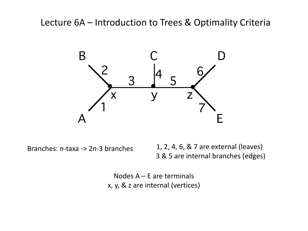
Lecture 6A Introduction to Trees & Optimality Criteria 1, 2, 4, 6, & 7 are external (leaves) 3 & 5 are internal branches (edges) Branches: n-taxa -> 2n-3 branches Nodes A E are terminals x, y, & z are internal (vertices)
Newick Format ((A,B),C,(D,E)). If we break branch 3, we have two sub-trees: (A,B) and (C,(D,E)).
Also note that there is free rotation around nodes: (1 2 3 4) (1 2 3 4) (1 2 3) (1 2 3) (1 2) (1 2) 5 5 1 1 2 2 3 3 4 4 1 1 2 2 3 3 4 4 5 5 = =
Growth of tree space. One of 15 possible 5-taxon trees. 7 * 15 = 105 possible 6-taxon trees.
The Scope of the Problem N (2i-5) B(N)= i=3 Taxa 3 4 5 6 7 8 9 10 22 50 100 1000 10 mil Unrooted Trees 1 3 15 105 945 10,395 135,135 2.027 X 10⁶ 3 X 10²³ 3 X 1074 2 X 1082 2 X 102,860 5 X 1068,667,340
II. Optimality Criteria A. Parsimony First, the score of a tree (i.e., its length) for the entire data set is given by: s Lt= wi li i=1 li is the length of character i when optimized on tree . wi is the weight we assign to character i.
The Fitch Algorithm (1971): state sets and accumulated lengths. Unordered states with equal transformation costs 1 G A 1 All changes are equivalent. 1 1 1 C T 1 Let s look at this tree, with the following distribution of states for character 1: G A C C 1 2 3
The Fitch Algorithm (1971): We erect a state set at each terminal node and assign an accumulated length of zero to terminal nodes. This is the minimum number of changes in the daughter subtree. {G}:0 {A}:0 {C}:0 {C}:0 1 2 3
The Fitch Algorithm (1971) 1 Form the intersection of the state sets of the two daughter nodes. If the intersection is non-empty, assign the set for the internal node equal to the intersection. The accumulated length of the internal node is the sum of those of the daughter nodes. 2 If the intersection is empty, we assign the union of the two daughter nodes to the state set for the internal node. The accumulated length is the sum of those of the daughter nodes plus one. {G}:0 {A}:0 {C}:0 {C}:0 non-empty empty Union: 0+0+1=1 {G,A}:1 {C}:0 empty Intersection: 0+0+0=0 Union: 1+0+1=2 {G,A,C}:2 So li= 2
Recall that the score of a tree (i.e., its length) for the entire data the (weighted) sum of the single-character lengths. s Lt= wi li i=1
Sankoff Algorithm Character-state vectors and step matrices. Step Matrix define ci,j 1 G A A C G T A -- 4 1 4 C 4 -- 4 1 G 1 4 -- 4 T 4 1 4 -- 4 4 4 4 C T 1 Step one: Fill in the character-state vectors for terminal nodes. Each cell is indexed by sk(i), the cost of having state i at node k.
A C G T A -- 4 1 4 C 4 -- 4 1 G 1 4 -- 4 T 4 1 4 -- Step two: Fill in vectors for other nodes, descending tree. Node 1 (k = 1): Node 2 (k = 2): s1(A) = cAG + cAA = 1 + 0 = 1, s2(A) = 4 + 4 = 8 s1(C) = cCG + cCA = 4 + 4 = 8, s2(C) = 0 + 0 = 0 s1(G) = cGG + cGA = 0 + 1 = 1, s2(G) = 4 + 4 = 8 s1(T) = cTG + cTA = 4 + 4 = 8 s2(T) = 1 + 1 = 2
For nodes below, we must calculate the cost for each possible state assignment for daughter nodes. From daughter node 1 From step matrix s3(A) = min[s1i + cAj] + min[s2i + cAj] = min[1,12,2,12] + min[8,4,9,6] = 1+4 = 5 s3(C) = min[s1i + cCj] + min[s2i + cCj] = min [5,8,5,9] + min[12,0,12,3] = 5+0 = 5 5 5 5 6 s3(G) = min[s1i + cGj] + min[s2i + cGj] = min [2,12,1,12] + min[9,4,8,6] = 1+4 = 5 A C G T A -- 4 1 4 C 4 -- 4 1 G 1 4 -- 4 T 4 1 4 -- s3(T) = min[s1i + cTj] + min[s2i + cTj] = min [5,9,5,8] + min[12,1,12,2] = 5+1 = 6 So, we fill in the character-state vector for node 3:
So, li = 5 Points to note: 1) Two types of weighting are possible: weighting of transformations within characters (which we demonstrated with the step matrix) and weighting among characters, which are reflected in the weighted sum of lengths across characters (wi). Lt= s wi li i=1 2) One can t compare tree lengths across weighting schemes. In the first example, with all transformations having the same cost, the length of the character on this tree was 2. In the second, with a 4:1 step matrix to weight transversions, the length was 5.


: state sets and accumulated")
:")
")
 for the")