Understanding Waveguiding Systems and Helmholtz Equation in Microwave Engineering

Waveguiding systems are essential in confining and channeling electromagnetic energy, with examples including rectangular and circular waveguides. The general notation for waveguiding systems involves wave propagation and transverse components. The Helmholtz Equation is a key concept in analyzing electromagnetic fields, providing insights into wave behavior in waveguides. By examining the equation and related laws, we gain a deeper understanding of waveguiding principles in microwave engineering.

• Waveguiding Systems
• Microwave Engineering
• Electromagnetic Energy
• Helmholtz Equation
• Wave Propagation

lili Follow

Uploaded on Jul 17, 2024 | 0 Views

Download Presentation

Please find below an Image/Link to download the presentation.

The content on the website is provided AS IS for your information and personal use only. It may not be sold, licensed, or shared on other websites without obtaining consent from the author. Download presentation by click this link. If you encounter any issues during the download, it is possible that the publisher has removed the file from their server.

Presentation Transcript

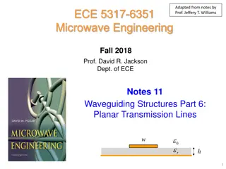
1. Adapted from notes by Prof. Jeffery T. Williams ECE 5317-6351 Microwave Engineering Fall 2019 Prof. David R. Jackson Dept. of ECE Notes 6 Waveguiding Structures Part 1: General Theory 1

2. Waveguide Introduction In general terms, a waveguiding system is a system that confines electromagnetic energy and channels it from one point to another. (This is opposed to a wireless system that uses antennas.) Examples Parallel plate waveguide Rectangular waveguide Circular waveguide Coax Twin lead (twisted pair) Printed circuit lines (e.g. microstrip) Transmission Lines Waveguides Optical fiber (dielectric waveguide) Note:In microwave engineering, the term waveguide is often used to mean rectangular or circular waveguide (i.e., a hollow pipe of metal). 2

3. General Notation for Waveguiding Systems Assume ej t time dependence and homogeneous source-free materials. Assume wave propagation in the z direction: z = = jk z z e e z = + = , j k j z c jk z C ( ) ( ) ( ) = + jk z Example of waveguiding system (a waveguide) z e x y , , , , E x y z e x y e z t z Transverse (x,y) components j c = j ( ) ( ) ( ) = + jk z z h x y , , , , c c H x y z h x y e = j z c t z tan c d Note: Lower case letters denote 2-D fields (the z term is suppressed). c 3

4. Helmholtz Equation = E j H = E v = + H j E J = 0 H ( ( j ) + = = = E j H ) j j E J ( ) + j E E j ( ) j j E Recall: c c = 2 k E where 2 2 k (complex) c 4

5. Helmholtz Equation = 2 E k E ( ) 2E Vector Laplacian definition: E E ( ) ( ) ( ) = + + where 2 2 2 2 x y z E E E E x y z ( ) = 2 2 E E k E = 2 2 v E k E + = 2 2 v E k E 5

6. Helmholtz Equation (cont.) So far we have: + = 2 2 v E k E Next, we examine the term on the right-hand side. 6

7. Helmholtz Equation (cont.) To do this, start with Ampere s law: = H j E c ( ) ( ) = = H j E c ( ) = = 0 j E c 0 0 E D = In the time-harmonic (sinusoidal) steady state, there can never be any volume charge density inside of a linear, homogeneous, isotropic, source-free region that obeys Ohm s law. 0 v 7

8. Helmholtz Equation (cont.) Hence, we have + = 2 2 0 E k E Vector Helmholtz equation 8

9. Helmholtz Equation (cont.) Similarly, for the magnetic field, we have = + H j E J = = = + H H j E E E ( ) + j ( ) j H j E Recall: c c ( ) ( ) ( = ) = H j E c ( )( j ) H j j H c ( ) k H ( )( ) = 2 H H j H c = 2 2 H 9

10. Helmholtz Equation (cont.) Hence, we have + = 2 2 0 H k H Vector Helmholtz equation 10

11. Helmholtz Equation (cont.) Summary + = 2 2 0 E k E + = 2 2 0 H k H Vector Helmholtz equation These equations are valid for a source-free, homogeneous, isotropic, linear material. 11

12. Helmholtz Equation (cont.) From the property of the vector Laplacian, we have + = 2 2 0 E k E z z + = 2 2 0 H k H z z Scalar Helmholtz equation ( ) ( ) ( ) = + + 2 2 2 2 x y z E E E E Recall: x y z 12

13. Field Representation Assume a guided wave with a field variation F(z) in the z direction of the form ( ) F z e = jk z z (This is a property of any guided wave.) Then all four of the transverse (x and y) field components can be expressed in terms of the two longitudinal ones: ( z E H ) , z 13

14. Field Representation: Proof jk z Assume a source-free region with a variation e z = = H j E E j H c Take (x,y,z) components H y E y = 4) jk H j E z = 1) jk E j H z z y c x z y x E x H x = 2) jk E j H z = 5) jk H j E z z x y z x c y E x E y H H y = y 3) j H x = y 6) j E x z z x 14

15. Field Representation: Proof (cont.) Combining 1) and 5): = 1 E y H x = jk jk H j H z z z z x x j c 2 z E y k H x k j H z z z x j c c E y H x = 2 2 z ( ) j jk k k H z z c z x 2 2 z 2 c k k k k c 1 k E y H x Cutoff wavenumber (real number, as discussed later) = H j jk z z x c z 2 c A similar derivation holds for the other three transverse field components. 15

16. Field Representation (cont.) Summary of Results E y H j = H k z z x c z 2 c k x These equations give the transverse field components in terms of the longitudinal components, Ezand Hz. E x H j = H k z z y c z 2 c k y = 2 2 k c E x H y j = + E k z z = 2 2 z k k k x z 2 c k c E y H x j = + E k z z y z 2 c k 16

17. Field Representation (cont.) Therefore, we only need to solve the Helmholtz equations for the longitudinal field components (Ez and Hz). + = 2 2 0 E k E z z + = 2 2 0 H k H z z From table , , , E E H H x y x y 17

18. Types of Waveguiding Systems Types of guided waves: TEMz ( R = TEMz: Ez = 0, Hz = 0 ) 0 TMz: Ez 0, Hz = 0 TEz: Ez = 0, Hz 0 Hybrid: Ez 0, Hz 0 TMz ,TEz ( PEC ) w Hybrid Hybrid r h Microstrip 18

19. Waveguides We assume that the boundary is PEC. We assume that the inside is filled with a homogenous isotropic linear material (could be air) An example of a waveguide (rectangular waveguide) Two types of modes: TEz ,TMz 19

20. Transverse Electric (TEz) Waves = 0 z E The electric field is transverse (perpendicular) to z. In general, Ex, Ey, Hx, Hy, Hz 0 To find the TEz field solutions (away from any sources), solve + = 2 2 ( ) 0 k H z or 2 2 2 + + + = 2 0 k H z 2 2 2 x y z 20

21. Transverse Electric (TEz) Waves (cont.) 2 2 2 + + + = 2 0 k H z 2 2 2 x y z Recall that the field solutions we seek are assumed to vary as ( ) F z e = jk z z jk z z = ( , , ) H x y z ( , ) h x y e z z 2 2 ( ) + + = 2 c 2 2 z 2 z 2 , 0 k k k k k h x y z 2 2 x y 2 c k 2 2 ( ) + + = 2 c , 0 k h x y z 2 2 x y 2 2 ( ) ( ) + = 2 c , , h x y k h x y z z 2 2 x y 21

22. Transverse Electric (TEz) Waves (cont.) 2 2 ( ) ( ) + = 2 c , , h x y k h x y z z 2 2 x y Change notation 2 2 ( ) ( ) + = , , x y x y 2 2 x y (2D Eigenvalue problem) ( ) , z h x y k = = eigenvalue = = eigenfunction 2 c For this type of eigenvalue problem, the eigenvalue is always real. (A proof of this may be found in the ECE 6340 notes.) We need to solve the eigenvalue problem subject to the appropriate boundary conditions. 22

23. Transverse Electric (TEz) Waves (cont.) 2 2 ( ) ( ) Neumann boundary condition (see below) + = 2 c , , h x y k h x y z z 2 2 x y A solution to the eigenvalue problem can always be found for a PEC boundary (proof omitted). Hence, TEz modes exist inside of a waveguide (conducting pipe). ( ) , zh x y z PEC c C c zh n = 0 C Neumann boundary condition 23

24. Transverse Electric (TEz) Waves (cont.) Once the solution for Hz is obtained, we use jk k jk k H x H y j k H y = = H E z z z x x 2 c 2 c j H x = = H E z z z y y 2 c 2 c k For a wave propagating in the positive z direction (top sign): E H E H = = y x k y x z For a wave propagating in the negative z direction (bottom sign): TE wave impedance E H E H = = y x k y x z Z TE k z 24

25. Transverse Electric (TEz) Waves (cont.) For a wave propagating in the positive z direction, we also have: ( ) ( ) ( ) = + xe x y ye , , , e x y x y t x y Recall: z e = ye xe t x y = = ( ) e Z h z e = = + yh xh Z x TE Z h y t TE y x e Z h y TE x TE t 1 = z e ( ) h t t Z TE Similarly, for a wave propagating in the negative z direction, 1 = z e ( ) h t t Z TE 25

26. Transverse Electric (TEz) Waves (cont.) Summarizing both cases, we have 1 ( ) ( ) ( ) = z e x y , , h x y t t Z TE + sign: wave propagating in the + z direction - sign: wave propagating in the - z direction 26

27. Transverse Magnetic (TMz) Waves = 0 H The magnetic field is transverse (perpendicular) to z. z In general, Ex, Ey, Ez ,Hx, Hy 0 To find the TEz field solutions (away from any sources), solve + = 2 2 ( ) 0 k E z or 2 2 2 + + + = 2 0 k E z 2 2 2 x y z 27

28. Transverse Magnetic (TMz) Waves (cont.) + + 2 2 2 + = 2 0 k E z 2 2 2 x y z Recall that the field solutions we seek are assumed to vary as ( , , ) z E x y z ( ) = jk z F z e z jk z z = ( , ) e x y e z 2 2 ( ) + + = 2 z 2 , 0 k k e x y 2 c 2 2 z k k k z 2 2 x y 2 c k 2 2 ( ) + + = 2 c , 0 k e x y z 2 2 x y 2 2 ( ) ( ) + = 2 c , , e x y k e x y z z 2 2 x y 28

29. Transverse Electric (TEz) Waves (cont.) 2 2 ( ) ( ) + = 2 c , , e x y k e x y z z 2 2 x y (Eigenvalue problem) ( ) = , = e x y eigenfunction z 2 c k eigenvalue We need to solve the eigenvalue problem subject to the appropriate boundary conditions. For this type of eigenvalue problem, the eigenvalue is always real. (A proof of this may be found in the ECE 6340 notes.) 29

30. Transverse Magnetic (TMz) Waves (cont.) 2 2 ( ) ( ) + = 2 c , , e x y k e x y Dirichlet boundary condition (see below) z z 2 2 x y A solution to the eigenvalue problem can always be found for a PEC boundary (proof omitted). Hence, TMz modes exist inside of a waveguide (conducting pipe). ( ) , ze x y z PEC c C c ze = 0 C Dirichlet boundary condition 30

31. Transverse Magnetic (TMz) Waves (cont.) Once the solution for Ez is obtained, we use j E y jk k jk k E x E y = = H c E z z z x x 2 c j 2 c k E x = = H c E z z z y y 2 c 2 c k For a wave propagating in the positive z direction (top sign): E H E H k = = y x z y x c For a wave propagating in the negative z direction (bottom sign): E H TM wave impedance E H k = = y x z k y x c Z z TM c 31

32. Transverse Magnetic (TMz) Waves (cont.) For a wave propagating in the positive z direction, we also have: ( ) ( ) ( ) = + xe x y ye , , , e x y x y t x y Recall: = ye xe z e t x y ( ) = = e Z h = = + yh xh z e Z x TM Z y h t TM y x e Z h y TM x TM t 1 = z ( ) h e t t Z TM Similarly, for a wave propagating in the negative z direction, 1 = z e ( ) h t t Z TM 32

33. Transverse Magnetic (TMz) Waves (cont.) Summarizing both cases, we have 1 ( ) ( ) ( ) = z e x y , , h x y t t Z TM + sign: wave propagating in the + z direction - sign: wave propagating in the - z direction 33

34. Transverse ElectroMagnetic (TEM) Waves = = 0, 0 E H z z In general, Ex, Ey, Hx, Hy 0 From the previous table for the transverse field components, all of them are equal to zero if Ez and Hz are both zero. E y H j = H k z z ck = x c z 2 Unless 2 c 0 k x E x H j = 2 c 2 2 z = 0 k k k For TEM waves H k z z y c z 2 c k y E x H y j Hence, we have = + E k z z x z 2 c k = = k k z c E y H x j = + E k z z y z 2 c k 34

35. Transverse ElectroMagnetic (TEM) Waves (cont.) ( ) ( ) ( ) = = jk z jkz , , , , H x y z h x y e h x y e z t From EM boundary conditions, we have: = n sJ H th so n ( ) ( ) e = jkz n , J h x y s t = z J J y s sz x The current flows purely in the z direction. 35

36. Transverse ElectroMagnetic (TEM) Waves (cont.) In a linear, isotropic, homogeneous source-free region, = 0 E In rectangular coordinates, we have E y E x E z y + + = 0 x z Notation: = + x y = 0 E t x y t ( ) ( ) = jk z , 0 e x y e z t t ( ) ( ) ( ) ( ) = jk z jk z , , 0 e e x y e x y e z z t t t ( ) ( ) = , 0 e x y t t Hence, we have ( ) ( ) = , 0 te x y t 36

37. Transverse ElectroMagnetic (TEM) Waves (cont.) Also, for the TEMzmode, we have from Faraday s law (taking the z component): ( ) ( z E z j = ) = = 0 H j H z Using the formula for the z component of the curl of E, we have: E x E y Note: y = 0 x = + x y Hence t x y ( ) ( ) ( ) = + e x xe x y ye , , , e x y x y e y y = t x y 0 x e x e y ( ) = y z , e x y x Hence, we have: t t ( ) ( ) = , 0 te x y t 37

38. Transverse ElectroMagnetic (TEM) Waves (cont.) ( ) ( ) = , 0 te x y t ( ) ( ) = , , e x y x y t t ( ) ( ) ( ) ( ) = = , 0 , 0 te x y x y t t t Hence ( ) = 2 t , 0 x y 38

39. Transverse ElectroMagnetic (TEM) Waves (cont.) Since the potential function that describes the electric field in the cross- sectional plane is two dimensional, we can drop the t subscript if we wish: ( ) = 2 , 0 x y ( ) = 2 , 0 x y Boundary Conditions: ( ( ) ) = = , x y conductor " " a a a b , x y conductor " " b b PEC conductors This is enough to make the potential function unique. Hence, the potential function is the same for DC as it is for a high- frequency microwave signal. The field of a TEM mode does not change shape with frequency: it has the same shape as a DC field. 39

40. Transverse ElectroMagnetic (TEM) Waves (cont.) Notes: A TEMz mode has an electric field that has exactly the same shape as a static (DC) field. (A similar proof holds for the magnetic field.) This implies that the C and L for the TEMz mode on a transmission line are independent of frequency. This also implies that the voltage drop between the two conductors of a transmission line carrying a TEMz mode is path independent. A TEMz mode requires two or more conductors: a static electric field cannot exist inside of a waveguide (hollow metal pipe) due to the Faraday cage effect. 40

41. Transverse ElectroMagnetic (TEM) Waves (cont.) For a TEM mode, both wave impedances are the same: = Recall: zk k = = = = = Z TE k k z c c k k = = = = = c Z z TM c c c c Note: is complex for lossy media. 41

42. TEM Solution Process A) Solve Laplace s equation subject to appropriate B.C.s.: ( ) , x y = 2 0 ( ) ( ) = B) Find the transverse electric field: , , te x y x y ( ) ( ) C) Find the total electric field: = = jk z , , , , E x y z e x y e k k z t z 1 ( ) D) Find the magnetic field: = z ; H E z propagating Note: The only frequency dependence is in the wavenumber kz = k. 42

43. Note on Lossy Transmission Line A TEM mode can have an arbitrary amount of dielectric loss. A TEM mode cannot have conductor loss. = J E Inside conductors: ( ) I z + + + + + + + - - - - - - - - - - ( ) V z If there is conductor loss, there must be an Ezfield. J E z z In practice, a small conductor loss will not change the shape of the fields too much, and the mode is approximately TEM. 43

44. Note on Lossy Transmission Line (cont.) If there is only dielectric loss (an exact TEM mode): ( )( ) = + j L G + j C R ( ) = = = jk jk k k z z ( )( ) = j L G + j C ) ( = ) ( )( ( ) = = jk j L G + j C 2 1 tan j 0 0 r r d j c Equate real and imaginary parts ( ) = 1 tan j j 0 0 r r d = LC ( ) 0 0 r r Note denotes real : r r ( )( ) L G ( ) = 2 tan 0 0 r r d 44

45. Note on Lossy Transmission Line (cont.) Equations for a TEM mode: = LC 0 0 r r ( )( ) L G ( ) = 2 tan 0 0 r r d ( ) ( ) ( ) 2 tan tan tan G C = = = 0 0 2 0 0 0 0 r r d r r d r r d LC LC 0 0 r r From these two equations we have: = LC 0 0 r r Note: These formulas were assumed previously in Notes 3. G C = tan d 45

46. Note on Lossy Transmission Line (cont.) This general formula accounts for both dielectric and conductor loss: ( )( ) = + j L G + j C R Dielectric loss Conductor loss When R is present the mode is not exactly TEM, but we usually ignore this. 46

47. Summary TEM Mode: ( ) = 1 tan j = = 0 E H rc r d z z = = r ( ) = = = 0 1 tan k k k k j c rc 0 0 z r rc r r d 1 ( ) = = ( ) ( ) 376.7303 0 = z e x y , , h x y 0 t t 0 47

48. Summary (cont.) Transmission line mode (approximate TEM mode): The mode requires two conductors. The mode is purely TEM only when R = 0. ( )( ) = = + j L G + j C jk R z = lossless L Z = LC 0 = 0 0 r r 0 0 r r = lossless / C Z 0 0 0 r r G C ( R ) R tan G C = = tan d d L C = z J J lossless Z s sz 0 48

49. Summary (cont.) TEz Mode: The mode can exist inside of a single pipe (waveguide). = 0, 0 E H z z ( ) = 2 2 c = = k k k 1 tan k k k j 0 0 r rc r r d z kc = real number (depends on geometry and mode number) 1 ( ) ( ) ( ) = z e x y , , h x y = Z t t Z TE k TE z ( ) ( ) k h x y = 2 t 2 c , , h x y z z 49

50. Summary (cont.) TMz Mode: The mode can exist inside a single pipe (waveguide). = 0, 0 H E z z ( ) = 2 2 c = = k k k 1 tan k k k j 0 0 r rc r r d z kc = real number (depends on geometry and mode number) 1 ( ) k ( ) ( ) = z e x y , , h x y = Z z t t Z TM TM ( ) ( ) k e x y = 2 t 2 c , , e x y z z 50