Fundamentals of Thermodynamic Property Relations

Determining thermodynamic properties is crucial for analysis, involving direct and derived properties expressed through formulations and relations. Partial derivatives, fundamental relations like the 1st and 2nd laws, and functions such as enthalpy, Helmholtz, and Gibbs are explored. Maxwell relations and generalized relations for changes in S, U, and H are discussed based on different pairs of independent variables.

• Thermodynamics
• Property Relations
• Partial Derivatives
• Fundamental Laws
• Enthalpy

philomena Follow

Uploaded on Jul 27, 2024 | 0 Views

Download Presentation

Please find below an Image/Link to download the presentation.

The content on the website is provided AS IS for your information and personal use only. It may not be sold, licensed, or shared on other websites without obtaining consent from the author. Download presentation by click this link. If you encounter any issues during the download, it is possible that the publisher has removed the file from their server.

Presentation Transcript

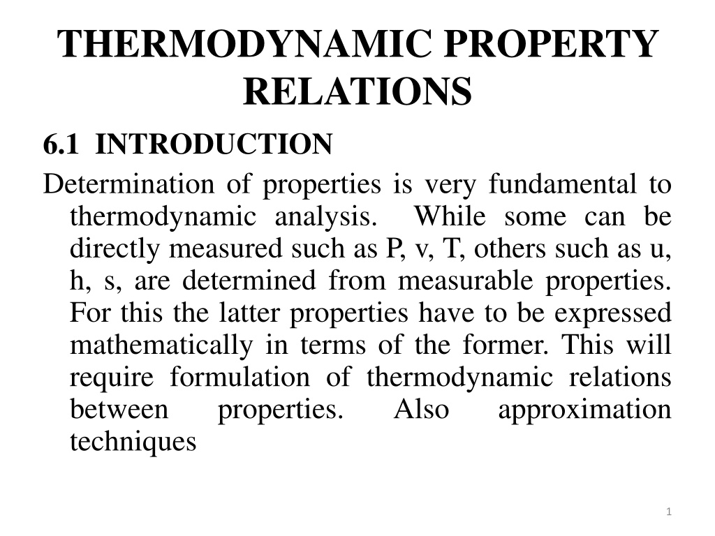
1. THERMODYNAMIC PROPERTY RELATIONS 6.1 INTRODUCTION Determination of properties is very fundamental to thermodynamic analysis. directly measured such as P, v, T, others such as u, h, s, are determined from measurable properties. For this the latter properties have to be expressed mathematically in terms of the former. This will require formulation of thermodynamic relations between properties. techniques While some can be Also approximation 1

2. will be developed as an alternative where sufficient data are not available to calculate properties. 6.2 FUNDAMENTALS OF PARTIAL DERIVATIVES Properties are point functions expressed as functions of two independent variables. This qualifies them to be exact differentials. The functional relationship may be expressed as x=x(y,z) or f(x,y,z) = 0 And the total differential is expressed as x dy y z x = + dx dz z y 2

3. fig-chp6\fig6.1.pptx shows the basis of partial derivative formulation. Rewriting as dx=Mdy + Ndz Exact differentials satisfy N z M = y y z They also satisfy the cyclic relation y z y z x y x z = 1 x 6.3 SOME FUNDAMENTAL RELATIONS 1st law: q=du+ w For a reversible process Tds=du+Pdv 1st Tds equation. More useful form: du=Tds-Pdv u=u(s,v) Using the definition of enthalpy h=u+Pv 3

4. Differentiation gives dh=du+Pdv+vdp or du +Pdv=dh-vdP Substitution in the 1st Tds equation gives the 2nd Tds equation : Tds=dh-vdP also dh=Tds+vdP h=h(s,P) Helmholtz function: a=u-Ts Differentiation gives da=du-Tds-sdT Using 1st Tds equation gives da=-Pdv-sdT a=a(T,v) Gibbs function: g=h-Ts Differentiation gives dg=dh-Tds-sdT Using the 2nd Tds equation gives dg=vdP-sdT g=g(T,P) 4

5. Applying the test of exactness gives the famous Maxwell relations T s v T P v P s v s = = = = P s T v T P s v s P v T P T Also u u h h = = = = T P T v s v s P v s P s a a g g = = = = P s v s v T P T T v T P 6.4 GENERALIZED RELATIONS FOR CHANGES IN S, U,AND H General equations indifferent to the type and phase of 5

6. of the substance are derived. Usually the two pairs of independent variables used are (T,v) and (T,P). Beginning with entropy as s=s(T,v) & 1st Tds equation s dT T T v dT c du v = dh = c s P = + = + v ds dv dT dv v T T v c dT p Also starting with s=s(T,P) & 2nd Tds equation + s s c v = = P ds dT dP dT dP T P T T P T P The following derived from Tds equations have been used. and T s s = = c T c T v P T 6 v P

7. With u=u(T,v) u u u = + = + du dT dv c dT dv v T v v v T T Using the 1st Tds equation and Maxwell relation = ,after integration = = du Tds pdv u Ts pv u s P = T P T P v v T T T v Substitution gives du = P + c dT T P dv v T v Similarly beginning with h=h(T,P) 7

8. h h h = + = + dh dT dP c dT dP P T P P P T T Using the 2nd Tds equation and Maxwell relation h s v = + = + T v T v P P T T T P Substitution gives v = + dh c dT v T dP P T P The determination of changes in s, u and h requires the knowledge of PvT behavior and experimental information on the relationship between specific heats and temperature. 8

9. 6.5 GENERALIZED RELATIONS FOR cP AND cv Two general relations derived were s T c = s = and c T v P T T v P Rewriting the ds equations c ds = P c v + = v P dT dv ds dT dP T T T T v P The test of exactness will give c v T 2 2 c P 2 P 2 = = v Or T v T v T T v v T 9

10. And c P T 2 2 v 2 c v 2 = = P Or T P T P T T P P T The above two equations give the variation of specific heats with volume and pressure at a given temperature. As an example, integration of the second equation from zero pressure gives 2 v 2 P = c c T dP 0 , P P T 0 P 10

11. where cP,0 is the zero pressure, or ideal gas, specific heat at the given temperature. The integration requires the knowledge of PvT behavior. If we equate the two ds expression (cP-cv)is determined as follows: c P c v + = v P dT dv dT dP T T T T v P c c P v = + P v or dT dv dP T T T v P Division by dP and imposing v=c yields T T c c v v P = = P v or c c T P v P T T T 11 v P P v

12. Using the cyclic relation for (P/ T)v will give v T c c 2 P = P v T v P T 1. cp- cv must always be positive or zero. It becomes zero at T=0 and 2. It also becomes zero when ( v/ T)P is ever zero. Eg. Maximum density of water at 4oC. 3. Since ( v/ T)P is very small for liquids and solids- gives cp-cv 0 4. For an ideal gas cp-cv =R 12

13. Other properties dealing with expansivity and compressibility are = 1 v exp volumetric ansion coefficien t 1 v T P v = K isothermal coefficien t of compressib ility T v P T Substitution of the above in the cp-cv expression gives vT c c = 2 P v K T The values of the coefficients are assumed to be constant in many calculations 13

14. Table 6.1 , KT, and at 1 bar vs. temperature for (a) copper and (b) water

15. 6.6 RESIDUAL PROPERTY FUNCTIONS This is an alternate method to determine changes in properties such as u, h, and s in states other than the ideal-gas state. For any specific property y a residual function yR is defined as yR y*- y or yR y - y* y is the desired value at T, P and y* is the property of an ideal gas at the same T, P (hypothetical). The change in property can be written as y2-y1 = (y2*-y2R)- (y1*- y1R) = y1R - y2R + (y2* - y1*) With the above definitions h can be determined as h ( ) h h ( h h 2 T , P 1 1 1 2 1 1 = = + + * * * P * P h ) h ( h ) 2 P T , 2 T , 2 T , 1 2 2 1 15

16. Referring to fig-chp6\fig6.2.pptx h ( h h a 1 2 = = + + h ) h ( h ) h ( h ) 1 b 2 b a Using the definition of residual functions T R R = + 2 h h h h c dT 2 1 1 2 , P o T 1 Similarly s can be determined as s = = + + * 1 * 2 * P * P s s s ( s ) s ( s ) s ( s ) 2 1 1 P T , 1 2 P T , 2 T T 1 2 2 2 1 1 The first two are the residual terms. c P T R R , = + P o 2 ln 2 s s s s dT R 2 1 1 2 T P T 1 1 16

17. Selecting state 1 as the reference state (ideal gas) at To and Po with ho* and so*, then the residual functions at one are zero. This will give T * = + R h h c dT h and , o P o T o c P T * , = + P T o R ln s s dT R s o P T o o Required are PvT data, ideal gas specific heat data and knowledge of the residual function. 17

18. 6.7 RESIDUAL PROPERTIES AND THE GIBBS FUNCTION Gibbs function given by dg=vdP-sdT is the convenient function to develop the residual function since it is expressed as g=g(P,T) and it will use those PvT relations that are explicit in v. Also dimensionless reduced function will be used as d(gR/RT) where v RT RT RT ( = = g d = g dg gdT h = = d dP dT 2 2 RT RT ) g h Ts and dg vdp v sdT were h 2 used * * * dP dT For an ideal gas RT RT RT 18

19. Subtraction of the first from the second gives the fundamental residual property relation as R R R g v h = d dP dT 2 RT RT RT Integrating at constant T from P=0 (ideal gas) to system pressure gives v RT R R 1 P g v P P = = = dP ( ) dP T C RT RT 0 0 The same equation at constant P gives hR as RT g T RT R R ( / ) h = = P C T 19 P

20. Also using gR=hR-TsR R R R R R ( / ) s h g g RT g = = T R RT RT T RT P Using the compressibility factor Z, v/RT=Z/P and substitution gives R g dP ( ) P = = 1 ( ) Z T C RT P RT 0 1 R R ( / ) h g Z P = = T T dP RT T T P 0 P P 20

21. This will give h = = R Z dP P = = T ( T C ) RT T P 0 P Similarly it can easily be shown Z T R R s dP dP ( ) P P = = 1 ( ) Z T C T P P 0 0 P For a two parameter equation in terms of reduced properties Z T RT P r c r R h P 2 = = r ln ( ) d P T C r r r T 0 21

22. Similarly R R R R s s h h dP dP ( ( ) ) P P = = = = r r 1 1 ( ( ) ) r r Z Z T T C C r r R R RT RT T c T c P P 0 0 r r r r The above require Z=Z(Pr,Tr)-charts A-39 and A-40 For internal energy one can start from (u=h-Pv) R R u h = = + + = = ( Z ) 1 ( T C ) RT RT 22

23. Using the three parameter equation with in the form of Z = Z(0) + Z(1) ) 0 ( ) 1 ( ) 0 ( ) 1 ( R R R R R R h h h s s s = + = + and R T R T R T R R R u c u c u c u u u Since ) 0 ( ) 1 ( Z Z Z = + T T T r r r P P P r r r Substitution in the hR/RuTc expression gives P r c T RT ) 0 ( ) 1 ( R h Z dP Z dP P P 2 2 = + r r r r T T r r P T P 0 0 r r r P r r 23

24. Similarly ) 0 ( R s Z dP P = + r ) 0 ( 1 r T Z r R T P 0 u r r P r ) 1 ( Z dP P + + r ) 0 ( 1 r T Z r T P 0 r r P r Tables A-26 through A-29 give the enthalpy and entropy residual functions. Example 6.1 example.docx 24

25. 6.8 RESIDUAL PROPERTIES AND THE HELMHOLTZ FUNCTION As most equations are of the form P=P(v,T), the Helmholtz function, a=a(v,T) also looks to be convenient to derive residual property relations. da=-Pdv-sdT or da=-Pdv at T=C * * v v = = = = * R a a a Pdv Pdv Pdv T C v v Infinite v indicates an ideal gas situation, hence RT * * v v = = = = * R a a a Pdv dv Pdv T C v v v 25

26. To eliminate the difficulty of infinite limits on the lower and upper bound add and subtract the integral of RT/v as follows: RT dv v RT RT RT * v = = * R a a a P dv dv dv v v v v v RT RT v * v v = = + ln P dv P dv RT * v v v v v Since Z was also defined as Z=vact/videal then Z=v/v* and this will give RT v = = + = * R ln a a a P dv RT Z T C v 26

27. ad To make it dimensionless divide by RuT a a T R u u * R 1 R T a v = = + = ln u P dv Z T C R T R T v u To get the residual functions for s and h, start with da==Pdv-sdT and noting that s=( a/ T)v, hence = * * ( ) s s a a v T Substitution of (a*-a) and taking the derivative with respect to T at constant v finally gives * 1 R s s P v = ln u dv R Z R R T v u u v 27

28. For enthalpy residual function, start with h = u + Pv = a+Ts +Pv since a=u-Ts Then hR = h*- h = (a*- a) + T(s*-s) + P*v*- Pv where P*v*=RT Substitutions for (a*-a) and (s*-s) will finally give T u * 1 h h P v = + 1 T P dv Z R R T T u v 28

29. Using g=a+Pv and u=h-Pv the residual functions for g and u can be determined from gR/RuT=aR/RuT + 1-Z and uR/RuT=hR/RuT + Z-1 All the above equations require P=P(v,T) 6.9 FLOW AVAILABILITY FROM RESIDUAL FUNCTIONS R=( *- )T,P=[(h*-h)-(ho*-ho)]-To[(s*-s)-(so*-so)] In dimensionless form * * R R * * * R T h h T s s h h s s = = o o o o o o RT RT RT T RT T c c c c c c , T P 29

30. This can be rearranged to give * R R R R R T T h s h s = = o o RT RT RT T R RT T R c c c c c c , T P , . T P oP T o Change in exergy will be R R R R h h s s 2 = + 2 1 2 1 RT RT 1 c o RT RT R R c c Example 6.2 example.docx 6.10 PROPERTIES OF THE SATURATION STATE Deals with liquid-vapor equilibrium of pure substances. Fundamental relationships among and approximate evaluation techniques for the basic properties P, T, u, h, s, a, and g are sought. 30

31. During phase change the heat supplied is called latent heat of evaporation, hfg and the change in entropy is given by hfg/Tsat. The combination gives hfg-Tsfg=0 or h-T s=0 (Phase change) From the definition of Gibbs function, g=h-Ts it follows gT = h - T s = 0 for a phase change or g =g or for the liquid-vapor phase gf=gg The equality of g for each phase is the criterion for phase quilibrium. From the relationship dg=vdP-sdT 31

32. We see that = g g = v and s P T T P Since v and s change discontinuously, the derivatives also change discontinuously (fig-chp6\fig6.3.pptx ). cP=T( s/ T)P in the mixture region is infinite while it has finite values at single phase points. For changes of dT and dP on the two phase (fig- chp6\fig6.4.pptx ) equilibrium system at the initial state (i) giL=giV. At the final equilibrium position giL +dgL=giV+dgV Thus for the change dT dgL = dgV 32

33. Using the expression for dg will give vL dP sL dT = vV dP sV dT And upon rearranging s dT s V L dP s fg = = V L v v v sat fg Since h = T s for a phase change h V L dP h ( h h fg = = = V L ) dT T v v T v Tv sat fg 33

34. The above is called Clapeyron equation- Used to determine enthalpy of vaporization. Applicable to sublimation and melting too. At low pressures ideal gas behavior can be considered and also vf<<vg = RT/P. This will give dT h P sat sat ln dP d P fg = = or h R fg 2 / 1 ( d ) RT T All the above are known as Clausius-Clapeyron equations. For small temperature change hfg remains approximately constant. Integration gives h P sat h 1 T 1 T P fg fg = + = sat 2 ln ln const or sat RT R P 34 2 1 1

35. The above equation shows linearity between ln Psat and 1/T for a small change in T at low pressures. Actual observation is that the linearity holds from the triple state to the critical state. This can be seen by inserting v=(Zg Zf)RT/P = Z (RT/P) in the Clapeyron equation and gives the modified Clapeyron equation as T RZ fg h 1 fg = sat ln d P d The ratio hfg/Zfg tends to remain constant with a minimum value at Tr= 0.85. Using Watson s hfg= (1-Tr)0.38 and Liley s Zfg= (1-Tr)0.38 35

36. Results in 1 dT dT = = = sat ln d P d 2 2 R T T T 6.10.1 Vapor-Pressure Correlations According to Clausius-Clapeyron equation vapor pressure can be fitted as B A P ln = = = sat tan / A cons t B h R fg T Modification is made on the above equation by using the normal boiling point Tb (at 1bar or 1 atm) and Tc and Pc to determine the constants A and B 36

37. = ln 1 ( A / ) P T T This will give B=Atb giving A=Tc ln Pc/(Tc-Tb) and the final equation becomes P ln T P ln b c b T = = sat 1 [ P ( bars , ) T ( K )] c c b T T T (reasonably accurate over a fairly wide range of temperatures) To improve the accuracy over a wider range of temperatures, the change incorporated. A Typical empirical vapor pressure correlations in use is in hfg must be B = + + + 2+ Psat ln ln A CT DT E T T 37

38. If a two parameter corresponding state is used on the Clausius-Clapeyron equation (ln Psat = A-B/T) It can easily be converted to = = sat r r T T ' 1 B sat ln ' ' 1 P A A r sat This gives a single straight line approximating the slope for all substances which is approximately true for simple fluids ( <0.05) as shown in fig- chp6\fig6.5.pptx . A second parameter is used to include the normal fluids in the form of Psat=f(Tsat, ) Pitzer s proposal r P = log log P sat + ) 0 ( (log ) r P r r T 38

39. The values for the right hand expressions are given in A-30 Other proposals of the form ln Prsat=f(0) + f(1) due to Lee-Kessler = . 1 92714 . 5 ln r T 09648 . 6 6 sat + 28862 ln 169347 . 0 P T T r r r 15 . 6875 T 6 + + 15 2518 . 13 4721 . ln 43577 . 0 T T r r r = / (recommended) where =-ln Pc-5.92714+6.09648 -1+1.28862 ln -0.169347 6 =15.2518-15.6875 -1 -13.4721 ln +0.43577 6 =Tb/Tc , Pc (atm) 39

40. Satisfies definition of ; curve passes through the critical state; curvature of the saturation line is zero at the critical state. Dong and Lienhard proposal: 1 T 3 6 sat 37270 . 5 = + . 7 ( 68769 . 3 + ln 1 49408 18177 . 11 P T T r r r r + 92998 . 17 ln ) T r Its major advantage over the Lee-Kessler equation is that it predicts better over a wider range of . Satisfies the definition of , as well as the critical state condition. 40

41. 6.10.2 Estimation of hfg Data Fishtine s correlation using the normal boiling point Tb given by h b b , fg b = 36 + ( . . ln ) ( / ) 6 8 31 k T J gmol and K T k=1 non-polar and 1<k<1.38 for polar and hydrogen bonded compounds Reidel s proposal (ln . , , P T RT c 930 0 . ) h 1 093 1 013 fg b = b r c ( , ) K bars . T , b r 41

42. Watsons for non associating liquids requiring a knowledge of hfg at one temperature . , r fg T h 0 38 h 1 T 2 fg , 2 = r 1 1 , 1 , Application of three-parameter corresponding states uses Clapeyron equation dP/dT= s/ v and since v=ZRT/P, then ZRT ln 1 dP R Z d P = = = ( ) r s Z Z Z g f ( / ) dT P T d T r r 42

43. Rewriting as 2 ( ) sat RT Z Z dP RTT Z dP g f = = r r h fg P dT P dT r r Pr=f(Tr, ) (slides 39 &40) and Table A-30 can be used for the above. Analytical correlation for Z from Haggenmacher (1946) is also useful 3 1 r T / 1 2 P = r Z Z g f 43

44. A suitable three-parameter (vaporization) correlation has the form s = sfg = sv(0) + sv(1) Table A-30 gives the right hand expressions. Since hfg=Tsfg then + + = = R ) 0 ( ) 1 ( v s s h RT v fg R (gives reasonable values for normal fluids) In dimensionless form R RT c r ) 0 ( ) 1 ( v h s s fg = = + + T v R 44

45. fig-chp6\fig6.6.pptx shows a linear function in the form of h + = fg ( ) a b fixed T r RT c According to Reid for 0.6 < Tr 1.0 the curves are well represented by h + = fg 354 . 456 . 0 0 . ( ) 95 . ( ) 7 08 1 10 1 T T r r RT c which is linear in for fixed Tr. 45

46. Finally a dimensionless correlation for temperature range Tc to triple state Tt according to Torquato and Stell and Torquato and Smith = fg t c h T T ( ) h T T T fg = c and ( ) T t = + + / 79 . 208 . 1 3 0 1 60176 . 45913 . 62671 . 0 3 4 + 2 3 89614 . 10643 . 31522 . 6 1 0 The equation represents the solid line of fig- chp6\fig6.7.pptx which fits the data for water. The above method requires hfg at the triple point (a major disadvantage). Example 6.3 example.docx 46

47. 6.10.3 Phase Equilibrium Properties from Equations of State For liquid vapor equilibrium gL=gV In terms of residual functions g g T R * * g g = R T u u L V If P(v,T) is given, then * * g g a a = + 1 Z R T R T u u 47

48. Using the expression for aR yields T R T R * 1 R T g g ( ) v = + ln 1 u v P dv Z Z u u As an example for RK fluid Z T R u * 1 + 1 g g b a b = ( ) ln 1ln 1 Z 5 . v bR T v u By first assuming Psat (using appropriate equations), RK equation (cubic in v) is solved for vf and vg and then Zg and Zf. Then check the equality of the phase equilibrium condition. If deviation is large, assume another Psat and repeat the procedure. 48

49. Then use R + 1 3 h a b = + ( ) 1ln 1 Z 5 . bR 2 R T T v u u to determine hgR and hfR. hfg= RuT(hgR hfR) Finally sfg=hfg/T For building up the table for hf, hg , sf ,sg in a saturation table requires a reference state. 49

50. 6.11 THE JOULE-THOMSON COEFFICIENT It has been seen that 1st law applied on throttling devices resulted in an isenthalpic process h1=h2. Also called Joule-Thomson effect. This usually results in a cold temperature, where the end result can be a two phase fluid and separation occurs. Other properties such as specific volumes, specific heats, and enthalpies may be evaluated from measurements of the Joule-Thomson effect. 50

Load More ...