Understanding Survival Analysis in Clinical Trials

Survival analysis plays a crucial role in analyzing data from randomized clinical trials, observational studies, and experiments. It involves estimating the survival function, conducting the log-rank test, and identifying when to use this analytical approach. Elements of survival experiments, standard notations for survival data, and practical applications in both RCTs and observational studies are explored in-depth.

Download Presentation

Please find below an Image/Link to download the presentation.
The content on the website is provided AS IS for your information and personal use only. It may not be sold, licensed, or shared on other websites without obtaining consent from the author. Download presentation by click this link. If you encounter any issues during the download, it is possible that the publisher has removed the file from their server.
E N D
Presentation Transcript
Survival Analysis for Randomized Clinical Trials Ziad Taib March 3, 2014 AstraZeneca.se
I The log-rank test 1. INTRODUCTION TO SURVIVAL TIME DATA 2. ESTIMATING THE SURVIVAL FUNCTION 3. THE LOG RANK TEST
Elements of Survival Experiments Event Definition (death, adverse events, ) Starting time Length of follow-up (equal length of follow-up, common stop time) Failure time (observed time of event since start of trial) Unobserved event time (censoring, no event recorded in the follow-up, early termination, etc) End of follow up time start Early termination event time
When to use survival analysis Examples Time to death or clinical endpoint Time in remission after treatment of CA Recidivism rate after alcohol treatment When one believes that 1+ explanatory variable(s) explains the differences in time to an event Especially when follow-up is incomplete or variable
Survival Analysis in RCT For survival analysis, the best observation plan is prospective. In clinical investigation, that is a randomized clinical trial (RCT). Random treatment assignments. Well-defined starting points. Substantial follow-up time. Exact time records of the interesting events.
Survival Analysis in Observational Studies Survival analysis can be used in observational studies (cohort, case control etc) as long as you recognize its limitations. Lack of causal interpretation. Unbalanced subject characteristics. Determination of the starting points. Lost of follow-up. Ascertainment of event times.
Standard Notation for Survival Data Ti-- Survival (failure) time Ci-- Censoring time Xi =min (Ti ,Ci)-- Observed time i =I(Ti Ci)-- Failure indicator: If the ith subjecthad an event before been censored, i=1, otherwise i=0. Zi(t) covariate vector at time t. Data: {Xi , i , Zi( ) }, where i=1,2, n.
Describing Survival Experiments Central idea: the event times are realizations of an unobserved stochastic process, that can be described by a probability distribution. Description of a probability distribution: 1. Cumulative distribution function 2. Survival function 3. Probability density function 4. Hazard function 5. Cumulative hazard function
Relationships Among Different Representations Given any one, we can recover the others. t ( ) 0 = = = ( ) 1 ( ) exp{ ( ) } S t P T t F t h u du t = ( ) ( ) H t h u du = ( ) log ( ) h t S t 0 t + Pr( | ) ( ) t T t t T t f t = = ( ) h t lim t ( ) t S t 0 t 0 = ( ) ( ) exp{ ( ) } f t h t h u du
Descriptive statistics Average survival Can we calculate this with censored data? Average hazard rate Total # of failures divided by observed survival time (units are therefore 1/t or 1/pt- yrs) An incidence rate, with a higher value indicating lower survival probability Provides an overall statistic only
Estimating the survival function There are two slightly different methods to create a survival curve. With the actuarial method, the x axis is divided up into regular intervals, perhaps months or years, and survival is calculated for each interval. With the Kaplan-Meier method, survival is recalculated every time a patient dies. This method is preferred, unless the number of patients is huge. The term life-table analysis is used inconsistently, but usually includes both methods.
Life Tables (no censoring) In survival analysis, the object of primary interest is the survival function S(t).Therefore we need to develop methods for estimating it in a good manner. The most obvious estimate is the empirical survival function: time 0 1 2 3 4 5 6 7 8 9 10 patients # with survival times larger tha n t ( ) t = S patients # Total 10 10 9 6 ( ) 0 ( ) 1 ( ) 2 ( ) 5 = = = = = = = 6 . 0 = 1 1 9 . 0 S S S S 10 10 10 10
Example: A RAT SURVIVAL STUDY In an experiment, 20 rats exposed to a particular type of radiation, were followed over time. The start time of follow-up was the same for each rat. This is an important difference from clinical studies where patients are recruited into the study over time and at the date of the analysis had been followed for different lengths of time. In this simple experiment all individuals have the same potential follow-up time. The potential follow- up time for each of the 20 rats is 5 days.
Survival Function for Ratsa [ P T = = ( ) [ ] ] S t P T t t
Proportion of rats dying on each of 5 days Survival Curve for Rat Study
Confidence Intervals for Survival Probabilities From above we see that the "cumulative" probability of surviving three days in the rat study is 0.25. We may want to report this probability along with its standard error. This sample proportion of 0.25 is based on 20 rats that started the study. If we assume that (i) each rat has the same unknown probability of surviving three days, S(3), and (ii) assume that the probability of one rat dying is not influenced by whether or not another rat dies, then we can use results associated with the binomial probability distribution to obtain the variance of this proportion. The variance is given by
(3) [1 (3)] 0.25 0.75 20 ) 3 ( N S S = = = [ (3)] 0.009375 VARIANCE S n ) 3 ( S S = ) 1 , 0 ( Z ) 3 ( S Var ( 1 ) ) 3 ( S ) 3 ( S ) 3 ( S Var 20 This can be used to test hypotheses about the theoretical probability of surviving three days as well as to construct confidence intervals. For example, the 95% confidence interval for is given by 0.25 +/- 1.96 x 0.094 or ( 0.060,0.440) We are 95% confident that the probability of surviving 3 days, meaning THREE OR MORE DAYS, lies between 0.060 and 0.440.
In general This approach has many drawbacks 1. Patients are recruited at different time periods 2. Some observations are censored 3. Patients can differ wrt many covariates 4. Continuous data is dicretised
Kaplan-Meier survival curves Also known as product-limit formula Accounts for censoring Generates the characteristic stair step survival curves Does not account for confounding or effect modification by other covariates Is that a problem?
In general 16 20 16 9 9 20 = = = = (2) [ 1] [ 2| 1] 0.45 S P T P T T The same as before! Similariliy = = (3) [ 1] 0.5625 9 16 [ 2| 1] [ 3| 2] S P T P T T P T T 0.80 16 20 0.5556 5 20 5 9 = = = 0.25
Censored Observations (Kaplan-Meier) We proceed as in the case without censoring ( ( ) i P P k S = 2 1 iP ) = ... Pr | 1 P T i T i i P k stands for the proportion of patients who survive day i among those who survive day i-1. Therefore it can be estimated according to ( Total number of patients) (Total - number of events during day 1) 1 P = ( Total number of patients) ( Number of Patients at risk day - i) (Total number of events during day i) = iP ( Number of Patients at risk day i)
K-M Estimate: General Formula Rank the survival times as t(1) t(2) t(n). Formula t t i i ) ( n n d ni patients at risk S ( i i = ) t di failures 19 20 = 1 0.95 = = P = = (1) (0) 0.95 0.95 S S P 1 1 19 17 20 19 17 19 = = 1 0.95 0.89464 = = (3) (0) 1 0.85 S S P P P = = 0.89474 1 3 3 PROC LIFETEST
Comparing Survival Functions Question: Did the treatment make a difference in the survival experience of the two groups? Hypothesis: H0: S1(t)=S2(t) for all t 0. Two tests often used : 1. Log-rank test (Mantel-Haenszel Test); 2. Cox regression
The Log-rank test During the th interval, let Nt be the number of patients at risk in the drug group at the beginning of the interval. Mt be the number of patients at risk in the placebo group at the beginning of the interval. At the number of events during the interval in the drug group Ct the number of events during the interval in the placebo group Tt = Nt + Mt
The Log-rank test Under H0, random allocation The above contingency table is a way of summarising the data at hand. Notice though that the marginals Nt and Mt are fixed. In principle the problem can be formulated as a formal test of H0: Drug has no effect hD(t) = hC(t) against H0: Drug is effective hD(t) = hK(t) = hK(t) / hD(t) = HR
This situation is similar to one where we have a total of Tt balls in an urn. These balls are of two different kinds D and C. Dtballs are drawn at random (those who experience events). We denote by At the number of balls of type D among the Dt drawn. Dt Tt = Nt + Mt
We can thus calculate probabilities of events like {At = a} using the hypergeometric distribution. M N t t D a a = = t ( ) P A a t T t D t The corresponding mean and variance are. ( ) T T T - D D N D N M A A = = = = 2 t ; ar t t t t t t t E V ( ) t t t 2 1 T t t t
The above can be used to derive the following test statistic where Nt and Mt are supposed to be large, which is often the case in RCT. A 2 t 2 t Z = ) 1 , 0 ( N t t Z and t t Assume now that we want to combine data from k successive such intervals. We can then define U according to ( ) = t 1 k = U tA And use the Mantel-Haensel statistic t 2 U = 2 1 Q Reject H0for large values of QM-H U M H Var
Some comments 1. The log-rank test is a significance test. It does not say anything about the size of the difference between the two groups. 2. The parameter can be used as measure of the size of that difference. It is also possible to compute confidence intervals for .
Further comments 3.Instead of QM-H we can formulate variants with weights 2 k ( ) = t A t t t = 1 k 2 1 Q under Ho. A = t 2 t Var t 1 1. t =1 M-H 2. t = Tt Gehan 1965 3. t = Tarone and Ware 1977 tT
A numerical example
Limitation of Kaplan-Meier curves What happens when you have several covariates that you believe contribute to survival? Example Smoking, hyperlipidemia, diabetes, hypertension, contribute to time to myocardial infarct Can use stratified K-M curves but the combinatorial complexity of more than two or three covariates prevents practical use Need another approach multivariate Cox proportional hazards model is most commonly used (think multivariate regression or logistic regression)
II Cox Regression Introduction to the proportional hazard model (PH) Partial likelihood Comparing two groups A numerical example Comparison with the log-rank test
The model = + + ( ) ( ) exp( ) h t h t x x 0 1 1 i i k ik Understanding baseline hazard h0(t) ( ) h t = + + exp[ ( ) ( )] i x x x x 1 1 1 i j k ik jk ( ) h t j
Cox Regression Model Proportional hazard. No specific distributional assumptions (but includes several important parametric models as special cases). Partial likelihood estimation (Semi- parametric in nature). Easy implementation (SAS procedure PHREG). Parametric approaches are an alternative, but they require stronger assumptions about h(t).
Cox proportional hazards model, continued Can handle both continuous and categorical predictor variables (think: logistic, linear regression) Without knowing baseline hazard ho(t), can still calculate coefficients for each covariate, and therefore hazard ratio Assumes multiplicative risk this is the proportional hazard assumption Can be compensated in part with interaction terms
Cox Regression In 1972 Cox suggested a model for survival data that would make it possible to take covariates into account. Up to then it was customary to discretise continuos variables and build subgroups. Cox idea was to model the hazard rate function T t t T t P + | ( = ) ( ) t h t t where h(t) is to be understood as an intensity i.e. a probability by time unit. Multiplied by time we get a probability. Think of the analogy with speed as distance by time unit. Multiplied by time we get distance.
Cox suggestion is to model h using T x x = ( ) = ( ) ; h t h t e i i 0 i ( ( ) T , ... , the parameter vector; 1 k ) Z Z = , ... , the covariate vector. Z Z i i 1 i ik where each parameter is a measure of the importance of the corresponding variable. A consequence of this is that two individuals with different covariate values will have hazard rate functions which differ by a multiplicative term which is the same for all values of t.
T x x = = ( ) ( ) ; , 1 ; 2 h t h t e i i i 0 i T x x ( ) ( ) h t e h t 1 1 T (x (x - - x x = = = ) 0 ; 1 e C 1 1 2 2 T x x ( ) h t ( ) h t ). e 2 2 2 0 = ( ) ( h t h t C 1 2 The covariates can be discrete, continuous or even categorical. It is also possible to generalise the model to allow time varying covariates.
Example Assume we have a situation with one covariate that takes two different values 0 and 1. This is the case when we wish to compare two treatments = = = ; 1 = ; k x x 1 = h2(t) 0; 0; x x ; 1 1 1 2 2 = ( ) ( ); h t h t 1 0 h1(t) = ( ) ( ). h t h t e 2 0 t
From the definition we see immediately that ( ) t S i Comments The baseline can be interpreted as the case corresponding to an individual with covariate values zero. t 0 ( ) h u du i = e t T 0 x x The name semi-parametric is due to the fact that we do not model h0 explicitly. Usual likelihood theory does not apply. i ( ) h u du e 0 = e T x x i e t 0 ( ) h u du 0 = e T e x x i = ( ) S t 0


")


 [1")


")