Understanding Survival Analysis in Medical Studies

Explore the key concepts of survival analysis, such as time-to-event data, censoring, and survivor functions. Learn how survival analysis methods estimate probabilities, compare survival rates between groups, and assess median survival times in medical research.

Download Presentation

Please find below an Image/Link to download the presentation.
The content on the website is provided AS IS for your information and personal use only. It may not be sold, licensed, or shared on other websites without obtaining consent from the author. Download presentation by click this link. If you encounter any issues during the download, it is possible that the publisher has removed the file from their server.
E N D
Presentation Transcript
Survival analysis Anne Segonds-Pichon v2020-07
Survival analysis Time to event data. Censoring. Survivor function Kaplan-Meier plot. Log-rank test. Hazard function and Hazard ratio .
Time to event data: examples Time to death. Time to progression of cancer. Time to development of diabetes. Time to recovery from diarrhea. Time to event data typically collected in cohort studies (time between study baseline and event of interest). clinical trials (time between randomisation and event of interest). Also known as survival data.
Features of time to event data Non-negative values. Not normally distributed (usually positively skewed). Event not usually observed for all individuals during the study. An observation is censored if individual does not experience event during the study. Censoring time: time from baseline/randomisation until latest date at which individual is known to be still alive and event-free.
Censoring Definition: Event of interest not observed for all individuals. Fixed censoring: event has not occurred when study has ended or data analysis is performed. Loss to follow-up: individual has been lost to follow-up (e.g. he/she no longer wishes to take part in study). Survival analysis methods make use of information from censored observations. Assume censoring is non-informative, i.e. if an individual is censored, his/her subsequent risk of the event of interest is unaffected.
Example of time to event data Weeks to death or censoring (*) in 20 adults with recurrent astrocytoma: Data reproduced from BMJ 2004; 328:1073.
Aims of survival analysis To estimate probability of not experiencing event of interest (not dying = surviving ) over any given time period (e.g. 5 year survival rate). To compare overall survival experience between different groups of individuals (e.g. between groups in a randomised clinical trial). Survivor function: Probability of not experiencing event of interest ( surviving ) up to time t. Example:
Estimating a survival rate Probability of surviving up to 2 years = 0.37.
Median survival time It is the time (expressed in months or years) when half the patients are expected to be alive. It means that the chance of surviving beyond that time is 50%. Median survival time = 1.4 years, since the probability of surviving up to 1.4 years is 0.5. 50% survival 1.4 years
Kaplan-Meier (KM) estimation of survivor function First death 20 individuals in study at t=0. First death at t=6 weeks. No individuals censored before t=6. Probability of death for each individual: 1/20=0.05 Therefore probability of surviving beyond t=6 is (1-0.05)=0.95=19/20. 1/20 19/20
K-M estimation of survivor function Second death 19 individuals in study between t=6 and t=13. Second death at t=13. No individuals censored between t=6 and t=13. Probability of death for each individual: 1/19=0.053 Therefore probability of surviving beyond t=13 is 0.95 x 0.947 =0.90. with 0.95=(1-(1/20)) and 0.947=(1-(1/19)) 18/19 19/20 1/19 1-(1/19)=18/19
K-M estimation of survivor function Third and fourth death 18 individuals in study between t=13 and t=21. Probability of death for each individual: 1/18=0.056 Probability of surviving beyond t=21 is 0.90 x (1-(1/18)) =0.85. From t=13: 0.95*0.947 17 individuals in study between t=21 and t=30. Probability of death for each individual: 1/17=0.059 Probability of surviving beyond t=30 is 0.85 x (1-(1/17)) =0.80. 1/19= 1/18= 1/17=
K-M estimation of survivor function Fifth and sixth death 16 individuals in study between t=30 and t=31. 1 individual censored at t=31. Probability of surviving beyond t=31 remains at 0.80. 15 individuals in study between t=31 and t=37. Probability of surviving beyond t=37 is 0.80 x (1-(1/15)) =0.747. 1/15=
K-M plot of survivor function Continue these calculations until reaching the longest event time. K-M plot drawn as a step function: First death: t=6, survival probability=0.95 Second death: t=13, survival probability=0.90 Third death: t=21, survival probability=0.85
K-M plot of survivor function Add ticks to indicate where censoring occurred. Data: tumours.slsx (astro data only)
Comparing 2 groups Weeks to death or censoring (*) in 20 adults with recurrent astrocytoma: Weeks to death or censoring (*) in 31 adults with recurrent glioblastoma: Data reproduced from BMJ 2004; 328:1073.
K-M plot of survivor function by tumour type Survival chances appear better in individuals with astrocytoma than with glioblastoma, but is the difference between groups statistically significant?
Comparing 2 samples Could compare median survival time, or probability of surviving up to any particular time. Better to use a test which compares survivor functions over whole follow-up period. Log rank test: tests null hypothesis of no difference between samples in probability of an event (death in this example) at any time point during follow-up. Log rank test statistic: based on calculating expected number of events that would occur under null hypothesis at each event time, and comparing to observed number of events. under null hypothesis has a Chi2 distribution with 1 degree of freedom.
Log rank test to compare 2 groups 31/51 20/51 Astro Glio Astro (31/50)*2 (19/50)*2 Log rank test statistic has a Chi2 distribution: =14 deaths =28 deaths
Log rank test Unlikely to detect a difference between Groups if survivor functions cross over during follow-up. Assumes non-informative censoring Can be extended to compare more than 2 groups. But Only provides a p-value, not an estimate of size of difference between groups or a confidence interval. Estimate of size of difference = Hazard Ratio
Hazard function Hazard is defined as the slope of the survival curve :a measure of how rapidly subjects are dying. Hazard function describes how hazard varies over time.
Hazard Ratio (HR) for comparing 2 samples Hazards may vary over time, but assume that HR is constant over time. The hazard ratio is not directly related to the ratio of median survival times. When comparing 2 groups (a and b): observed events (deaths) in each group: Oa and Ob, expected events (deaths) in each group: Ea and Eb, assuming a null hypothesis of no difference in survival. HR= (Oa/Ea)/(Ob/Eb) No assumption is needed about shape of hazard functions or underlying distribution of time to event data. HR is obtained from Cox regression
Hazard Ratio (HR) Data: tumours.xlsx HR = 2.3 (95% CI [1.32;4.44]) At any point in time, hazard (i.e. instantaneous rate) of dying in individuals with recurrent glioblastoma is 2.3 times higher than in individuals with recurrent astrocytoma.
Comparing more than 2 samples Issue with GraphPad: cannot compare more than 2 groups directly As in: does not run post-hoc pairwise comparisons So how do we do it? Step 1: All groups comparisons (equivalent omnibus step in ANOVA) Step 2: Make all pairwise comparisons of interest Step 3: Apply Bonferroni correction Example dataset: Lung infection Mice are infected with Streptococcus pneumoniae 3 groups: Control, treatment 1 and treatment 2
Comparing more than 2 groups Step 1: All groups comparisons There is an overall difference in survival between the 3 groups but which group is different from which?
Comparing more than 2 groups Step 2: Make all pairwise comparisons of interest T1 vs. T2 Control vs. T1 Control vs. T2 Adjusted p-value = 0.5394 Adjusted p-value = 0.4101 Adjusted p-value = 0.0405 Step 3: Apply Bonferroni correction: 0.05/3=0.06 or initial p-values*3
Comparing more than 2 groups At any point in time, hazard of dying in mice with lung infection is: almost 2 times higher in the control than in the treatment 1 group (p=0.54) 3.6 times higher in the control than in the treatment 1 group (p=0.04)


 estimation of survivor function")


")
")