Efficient Techniques for Handling Missing Data Values
Explore effective methods for handling missing data values, including what not to do and how to improve imputation techniques. Discover the drawbacks of common approaches and learn better strategies to enhance accuracy and reduce bias in data analysis.

Download Presentation

Please find below an Image/Link to download the presentation.
The content on the website is provided AS IS for your information and personal use only. It may not be sold, licensed, or shared on other websites without obtaining consent from the author. Download presentation by click this link. If you encounter any issues during the download, it is possible that the publisher has removed the file from their server.
E N D
Presentation Transcript
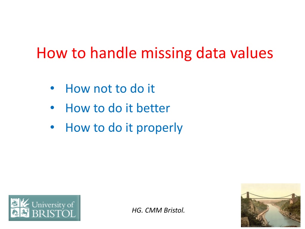
How to handle missing data values How not to do it How to do it better How to do it properly HG. CMM Bristol.
Information about missing data techniques www.missingdata.org.uk (free to register) Software: REALCOM-IMPUTE: free 2-level, general but slow STATJR: General n-level (2-level free) fast To illustrate concepts let s consider a simple example: 07/10/2024 2
Simple regression: y on x ??= ? + ???+ ???,?,????????? ?????? For example: y x 31.5 * 22.3 3.2 * 1.9 . . . . So let s generate a dataset large enough so we can illustrate matters without having to go through tedious simulations. 07/10/2024 3
The dataset ? ?~N i.e. regression is: 0 0 1 (1) , 0.5 1 ?2= 0.75 ( ? = ???(??)/???(?)) ? = 0.5? Simulate 100,000 pairs of values and estimate regression: We get ? = 0.502 (0.00274) ?2= 0.751 Set about 20% of y s missing at random 20% x s missing but not at random. Pr(? ???????) |y|) We ll apply some popular (intuitive?) procedures Note that if both missing (~4%) there is no information so delete these, leaving 96028 cases. Fundamental idea is that of Imputation. This silence for my sin you did impute, Which shall be most my glory, being dumb; W.S. Sonnet 83. 07/10/2024 4
What not to do - 1 Calculate mean of observed and substitute for missing We get estimates (standard error in brackets); ? = 0.455(0.00275) ?2= 0.632 This is biased. Also note standard error wrong since ~36% values are imputed and not actually observed so estimate too small. Correct standard error is elusive. 07/10/2024 5
What not to do - 2 Use observed complete records to predict y|? & ?|? and use predicted values to plug in for missing. Prediction imputation We get estimates (standard error in brackets); ? = 0.573 (0.00264) ?2= 0.591 Parameters still biased as is standard error. Now use just the complete records ? = 0.569 (0.00357) ?2= 0.851 This is popular because simple but large bias still because complete records not a random sample But, if you have complete cases as a random sample we get; ? = 0.500 (0.00341) ?2= 0.748 So now unbiased but standard error larger than for full data since smaller sample. 07/10/2024 6
How to do it better - 3 2, ??2,??? biased. For plug in and prediction imputation ?? So for rgression impute let s add a random variable on to each imputed (predicted) value, drawn from the regression residual distributions, i.e. ? ? ? & ?(?|?) We now get estimates (standard error in brackets); ? = 0.502 (0.00279) ?2= 0.754 Bias now virtually gone but standard error still too small since takes no account of fact that imputed values are derived from data and not observed. We call this random regression imputation 07/10/2024 7
How to do it better - 4 Hot decking as enjoyed by survey analysts. For each missing x (or y) find the set of y s (x s) that are similar to the value of y say y* (x say x*) associated with the missing x (y). Issue about how to define similar in present case we shall take all those y s in the range ( ) 0.1 but we can do sensitivity analyses. For that set of y s select one at random or if you want to be sophisticated sample according to the distance from y*. This then becomes the imputed value. Results when it works similar to random regression imputation In practice the choice of range is crucial and for several variables we may not be able to find suitable pools of records from which to randomly select y 07/10/2024 8
How to do it better - 4 ctd. So: when missing not random the only procedure that gives unbiased parameter estimates, but incorrect standard errors is random imputation. When missingness random complete case analysis and random imputation are unbiased; the former is inefficient, the latter gives incorrect standard error. 07/10/2024 9
How to do it properly Known as multiple imputation it basically does a random imputation but repeats it independently n times, where n is a suitably large number traditionally 5 but more realistically up to 20. An MCMC chain is typically used. We therefore obtain n estimates of ?,?2, and these are averaged using Rubin s rules - to obtain final values together with consistent standard error estimates. For n=5 we get ? = 0.503 (0.00290) ?2= 0.752 And we now have unbiased estimates with correct standard error and we see that it is relatively efficient This is then the basis for a more general implementation (multilevel with mixed variable types) as in REALCOM and STATJR. Finally a fully Bayesian procedure has been developed that is fast, very general and will also become available in STATJR 07/10/2024 10
A general approach We have a multilevel MOI with a response (possibly >1) and covariates possibly at several levels. We take all the variables at each level and make a multivariate response model with complete variables either as responses or covariates. We finish up with a multilevel multivariate response model and at each higher level we allow the responses at that level to correlate with random effects derived from a lower level. At this point we can include auxiliaries that are not in the MOI but might be associated with the propensity to be missing thus improving our ability to satisfy the missing at random (MAR) i.e. randomly missing given the other variables in the MOI. This assumption is needed. Within an MCMC chain we produce n complete data sets and fit the MOI to each one. Then we combine: 07/10/2024 11
Combining MOIs Using Rubins Rules Take the average estimates 1 1 N N = n = n ) ( = = 2 ( ) n ) n Within ( ESE ( ) N P 1 1 Between-imputation average of variances 1 2 N = n ) = ( ) n Between ( ( ) 1 N N 1 Combine + 1 N ) ) ) = + var ( Within ( 1 Between ( 07/10/2024 12
Handling a mixture of variable types All of this so far assumes normality. What if we also have categorical data? Key reference: Goldstein, H., Carpenter, J., Kenward, M. and Levin, K. (2009). Multilevel models with multivariate mixed response types. Statistical Modelling, 9,3, 173-197. Essentially works by assuming underlying normal distributions that generate discrete variables via thresholds, e.g. probit model for binary data. STATJR software: 2-level version freely downloadable from CMM. Note that while STATA (MICE) can handle mixed variable types it cannot handle higher level variables and doesn t have a strong methodological foundation. Most other software assumes normality throughout. 07/10/2024 13
Further developments Existing MI methods cannot properly handle interactions including power terms New development: (Goldstein, H., Carpenter, J. R. and Browne, W. J. (2013), JRSSA doi: 10.1111/rssa.12022) Allows interactions and polynomials: At each iteration of an MCMC chain we fit IM the MOI together based on joint likelihood. This gives a single MOI chain that can be used for inferences in the usual ways. Avoids a 2-stage procedure and allows sensitive data diagnostics. 07/10/2024 14