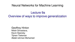
Mini-Batch Gradient Descent in Neural Networks

In this lecture by Geoffrey Hinton, Nitish Srivastava, and Kevin Swersky, an overview of mini-batch gradient descent is provided. The discussion includes the error surfaces for linear neurons, convergence speed in quadratic bowls, challenges with learning rates, comparison with stochastic gradient descent, and strategies for optimizing learning algorithms, particularly in large neural networks.

Download Presentation

Please find below an Image/Link to download the presentation.
The content on the website is provided AS IS for your information and personal use only. It may not be sold, licensed, or shared on other websites without obtaining consent from the author. Download presentation by click this link. If you encounter any issues during the download, it is possible that the publisher has removed the file from their server.
E N D
Presentation Transcript
Neural Networks for Machine Learning Lecture 6a Overview of mini-batch gradient descent Geoffrey Hinton with Nitish Srivastava Kevin Swersky
Reminder: The error surface for a linear neuron The error surface lies in a space with a horizontal axis for each weight and one vertical axis for the error. For a linear neuron with a squared error, it is a quadratic bowl. Vertical cross-sections are parabolas. Horizontal cross-sections are ellipses. For multi-layer, non-linear nets the error surface is much more complicated. But locally, a piece of a quadratic bowl is usually a very good approximation. E w1 w2
Convergence speed of full batch learning when the error surface is a quadratic bowl Going downhill reduces the error, but the direction of steepest descent does not point at the minimum unless the ellipse is a circle. The gradient is big in the direction in which we only want to travel a small distance. The gradient is small in the direction in which we want to travel a large distance. Even for non-linear multi-layer nets, the error surface is locally quadratic, so the same speed issues apply.
How the learning goes wrong If the learning rate is big, the weights slosh to and fro across the ravine. If the learning rate is too big, this oscillation diverges. What we would like to achieve: Move quickly in directions with small but consistent gradients. Move slowly in directions with big but inconsistent gradients. E w
Stochastic gradient descent Mini-batches are usually better than online. Less computation is used updating the weights. Computing the gradient for many cases simultaneously uses matrix-matrix multiplies which are very efficient, especially on GPUs Mini-batches need to be balanced for classes If the dataset is highly redundant, the gradient on the first half is almost identical to the gradient on the second half. So instead of computing the full gradient, update the weights using the gradient on the first half and then get a gradient for the new weights on the second half. The extreme version of this approach updates weights after each case. Its called online .
Two types of learning algorithm If we use the full gradient computed from all the training cases, there are many clever ways to speed up learning (e.g. non-linear conjugate gradient). The optimization community has studied the general problem of optimizing smooth non-linear functions for many years. Multilayer neural nets are not typical of the problems they study so their methods may need a lot of adaptation. For large neural networks with very large and highly redundant training sets, it is nearly always best to use mini-batch learning. The mini-batches may need to be quite big when adapting fancy methods. Big mini-batches are more computationally efficient.
A basic mini-batch gradient descent algorithm Guess an initial learning rate. If the error keeps getting worse or oscillates wildly, reduce the learning rate. If the error is falling fairly consistently but slowly, increase the learning rate. Write a simple program to automate this way of adjusting the learning rate. Towards the end of mini-batch learning it nearly always helps to turn down the learning rate. This removes fluctuations in the final weights caused by the variations between mini- batches. Turn down the learning rate when the error stops decreasing. Use the error on a separate validation set
Neural Networks for Machine Learning Lecture 6b A bag of tricks for mini-batch gradient descent Geoffrey Hinton with Nitish Srivastava Kevin Swersky
Be careful about turning down the learning rate Turning down the learning rate reduces the random fluctuations in the error due to the different gradients on different mini-batches. So we get a quick win. But then we get slower learning. Don t turn down the learning rate too soon! reduce learning rate error epoch
Initializing the weights If two hidden units have exactly the same bias and exactly the same incoming and outgoing weights, they will always get exactly the same gradient. So they can never learn to be different features. We break symmetry by initializing the weights to have small random values. If a hidden unit has a big fan-in, small changes on many of its incoming weights can cause the learning to overshoot. We generally want smaller incoming weights when the fan-in is big, so initialize the weights to be proportional to sqrt(fan-in). We can also scale the learning rate the same way.
Shifting the inputs color indicates training case w1 w2 When using steepest descent, shifting the input values makes a big difference. It usually helps to transform each component of the input vector so that it has zero mean over the whole training set. The hypberbolic tangent (which is 2*logistic -1) produces hidden activations that are roughly zero mean. In this respect its better than the logistic. 101, 101 2 101, 99 0 gives error surface 1, 1 2 1, -1 0 gives error surface
Scaling the inputs color indicates weight axis w1 w2 When using steepest descent, scaling the input values makes a big difference. It usually helps to transform each component of the input vector so that it has unit variance over the whole training set. 0.1, 10 2 0.1, -10 0 gives error surface 1, 1 2 1, -1 0 gives error surface
A more thorough method: Decorrelate the input components For a linear neuron, we get a big win by decorrelating each component of the input from the other input components. There are several different ways to decorrelate inputs. A reasonable method is to use Principal Components Analysis. Drop the principal components with the smallest eigenvalues. This achieves some dimensionality reduction. Divide the remaining principal components by the square roots of their eigenvalues. For a linear neuron, this converts an axis aligned elliptical error surface into a circular one. For a circular error surface, the gradient points straight towards the minimum.
Common problems that occur in multilayer networks In classification networks that use a squared error or a cross-entropy error, the best guessing strategy is to make each output unit always produce an output equal to the proportion of time it should be a 1. The network finds this strategy quickly and may take a long time to improve on it by making use of the input. This is another plateau that looks like a local minimum. If we start with a very big learning rate, the weights of each hidden unit will all become very big and positive or very big and negative. The error derivatives for the hidden units will all become tiny and the error will not decrease. This is usually a plateau, but people often mistake it for a local minimum.
Four ways to speed up mini-batch learning rmsprop: Divide the learning rate for a weight by a running average of the magnitudes of recent gradients for that weight. This is the mini-batch version of just using the sign of the gradient. Take a fancy method from the optimization literature that makes use of curvature information (not this lecture) Adapt it to work for neural nets Adapt it to work for mini-batches. Use momentum Instead of using the gradient to change the position of the weight particle , use it to change the velocity. Use separate adaptive learning rates for each parameter Slowly adjust the rate using the consistency of the gradient for that parameter.
Neural Networks for Machine Learning Lecture 6c The momentum method Geoffrey Hinton with Nitish Srivastava Kevin Swersky
The intuition behind the momentum method It damps oscillations in directions of high curvature by combining gradients with opposite signs. It builds up speed in directions with a gentle but consistent gradient. Imagine a ball on the error surface. The location of the ball in the horizontal plane represents the weight vector. The ball starts off by following the gradient, but once it has velocity, it no longer does steepest descent. Its momentum makes it keep going in the previous direction.
The equations of the momentum method The effect of the gradient is to increment the previous velocity. The velocity also decays by which is slightly less then 1. v(t)=a v(t-1)-e E w(t) Dw(t)=v(t) The weight change is equal to the current velocity. =a v(t-1)-e E w(t) The weight change can be expressed in terms of the previous weight change and the current gradient. =a Dw(t-1)-e E w(t)
The behavior of the momentum method At the beginning of learning there may be very large gradients. So it pays to use a small momentum (e.g. 0.5). Once the large gradients have disappeared and the weights are stuck in a ravine the momentum can be smoothly raised to its final value (e.g. 0.9 or even 0.99) This allows us to learn at a rate that would cause divergent oscillations without the momentum. If the error surface is a tilted plane, the ball reaches a terminal velocity. If the momentum is close to 1, this is much faster than simple gradient descent. -e E w 1 v( )= 1-a
A better type of momentum (Nesterov 1983) The standard momentum method first computes the gradient at the current location and then takes a big jump in the direction of the updated accumulated gradient. Ilya Sutskever (2012 unpublished) suggested a new form of momentum that often works better. Inspired by the Nesterov method for optimizing convex functions. First make a big jump in the direction of the previous accumulated gradient. Then measure the gradient where you end up and make a correction. Its better to correct a mistake after you have made it!
A picture of the Nesterov method First make a big jump in the direction of the previous accumulated gradient. Then measure the gradient where you end up and make a correction. brown vector = jump, red vector = correction, green vector = accumulated gradient blue vectors = standard momentum
Neural Networks for Machine Learning Lecture 6d A separate, adaptive learning rate for each connection Geoffrey Hinton with Nitish Srivastava Kevin Swersky
The intuition behind separate adaptive learning rates In a multilayer net, the appropriate learning rates can vary widely between weights: The magnitudes of the gradients are often very different for different layers, especially if the initial weights are small. The fan-in of a unit determines the size of the overshoot effects caused by simultaneously changing many of the incoming weights of a unit to correct the same error. So use a global learning rate (set by hand) multiplied by an appropriate local gain that is determined empirically for each weight. Gradients can get very small in the early layers of very deep nets. The fan-in often varies widely between layers.
One way to determine the individual learning rates E wij Start with a local gain of 1 for every weight. Increase the local gain if the gradient for that weight does not change sign. Use small additive increases and multiplicative decreases (for mini-batch) This ensures that big gains decay rapidly when oscillations start. If the gradient is totally random the gain will hover around 1 when we increase by plus half the time and decrease by times half the time. Dwij=-e gij > 0 E wij gij(t)= gij(t-1)+.05 gij(t)= gij(t-1)*.95 (t) E wij (t-1) if then d1-d else
Tricks for making adaptive learning rates work better Adaptive learning rates can be combined with momentum. Use the agreement in sign between the current gradient for a weight and the velocity for that weight (Jacobs, 1989). Adaptive learning rates only deal with axis-aligned effects. Momentum does not care about the alignment of the axes. Limit the gains to lie in some reasonable range e.g. [0.1, 10] or [.01, 100] Use full batch learning or big mini- batches This ensures that changes in the sign of the gradient are not mainly due to the sampling error of a mini- batch.
Neural Networks for Machine Learning Lecture 6e rmsprop: Divide the gradient by a running average of its recent magnitude Geoffrey Hinton with Nitish Srivastava Kevin Swersky
rprop: Using only the sign of the gradient The magnitude of the gradient can be very different for different weights and can change during learning. This makes it hard to choose a single global learning rate. For full batch learning, we can deal with this variation by only using the sign of the gradient. The weight updates are all of the same magnitude. This escapes from plateaus with tiny gradients quickly. rprop: This combines the idea of only using the sign of the gradient with the idea of adapting the step size separately for each weight. Increase the step size for a weight multiplicatively (e.g. times 1.2) if the signs of its last two gradients agree. Otherwise decrease the step size multiplicatively (e.g. times 0.5). Limit the step sizes to be less than 50 and more than a millionth (Mike Shuster s advice).
Why rprop does not work with mini-batches The idea behind stochastic gradient descent is that when the learning rate is small, it averages the gradients over successive mini- batches. Consider a weight that gets a gradient of +0.1 on nine mini- batches and a gradient of -0.9 on the tenth mini-batch. We want this weight to stay roughly where it is. rprop would increment the weight nine times and decrement it once by about the same amount (assuming any adaptation of the step sizes is small on this time-scale). So the weight would grow a lot. Is there a way to combine: The robustness of rprop. The efficiency of mini-batches. The effective averaging of gradients over mini-batches.
rmsprop: A mini-batch version of rprop rprop is equivalent to using the gradient but also dividing by the size of the gradient. The problem with mini-batch rprop is that we divide by a different number for each mini-batch. So why not force the number we divide by to be very similar for adjacent mini-batches? rmsprop: Keep a moving average of the squared gradient for each weight MeanSquare(w, t)= 0.9 MeanSquare(w, t-1)+ 0.1 E w(t) MeanSquare(w, t) ( ) 2 Dividing the gradient by makes the learning work much better (Tijmen Tieleman, unpublished).
Further developments of rmsprop Combining rmsprop with standard momentum Momentum does not help as much as it normally does. Needs more investigation. Combining rmsprop with Nesterov momentum (Sutskever 2012) It works best if the RMS of the recent gradients is used to divide the correction rather than the jump in the direction of accumulated corrections. Combining rmsprop with adaptive learning rates for each connection Needs more investigation. Other methods related to rmsprop Yann LeCun sgroup has a fancy version in No more pesky learning rates
Summary of learning methods for neural networks Neural nets differ a lot: Very deep nets (especially ones with narrow bottlenecks). Recurrent nets. Wide shallow nets. Tasks differ a lot: Some require very accurate weights, some don t. Some have many very rare cases (e.g. words). For small datasets (e.g. 10,000 cases) or bigger datasets without much redundancy, use a full-batch method. Conjugate gradient, LBFGS ... adaptive learning rates, rprop ... For big, redundant datasets use mini- batches. Try gradient descent with momentum. Try rmsprop (with momentum ?) Try LeCun s latest recipe. Why there is no simple recipe:


")