Understanding Principal Components Analysis (PCA) and Autoencoders in Neural Networks

Principal Components Analysis (PCA) is a technique that extracts important features from high-dimensional data by finding orthogonal directions of maximum variance. It aims to represent data in a lower-dimensional subspace while minimizing reconstruction error. Autoencoders, on the other hand, are neural networks used for non-linear dimensionality reduction. By using backpropagation, PCA concepts can be implemented within autoencoders efficiently. Deep autoencoders further enhance this by allowing flexible mappings for non-linear dimensionality reduction.

Download Presentation

Please find below an Image/Link to download the presentation.
The content on the website is provided AS IS for your information and personal use only. It may not be sold, licensed, or shared on other websites without obtaining consent from the author. Download presentation by click this link. If you encounter any issues during the download, it is possible that the publisher has removed the file from their server.
E N D
Presentation Transcript
Neural Networks for Machine Learning Lecture 15a From Principal Components Analysis to Autoencoders Geoffrey Hinton Nitish Srivastava, Kevin Swersky Tijmen Tieleman Abdel-rahman Mohamed
Principal Components Analysis This takes N-dimensional data and finds the M orthogonal directions in which the data have the most variance. These M principal directions form a lower-dimensional subspace. We can represent an N-dimensional datapoint by its projections onto the M principal directions. This loses all information about where the datapoint is located in the remaining orthogonal directions. We reconstruct by using the mean value (over all the data) on the N- M directions that are not represented. The reconstruction error is the sum over all these unrepresented directions of the squared differences of the datapoint from the mean.
A picture of PCA with N=2 and M=1 The red point is represented by the green point. The reconstruction of the red point has an error equal to the squared distance between red and green points. direction of first principal component i.e. direction of greatest variance
Using backpropagation to implement PCA inefficiently Try to make the output be the same as the input in a network with a central bottleneck. If the hidden and output layers are linear, it will learn hidden units that are a linear function of the data and minimize the squared reconstruction error. This is exactly what PCA does. The M hidden units will span the same space as the first M components found by PCA Their weight vectors may not be orthogonal. They will tend to have equal variances. output vector code input vector The activities of the hidden units in the bottleneck form an efficient code.
Using backpropagation to generalize PCA With non-linear layers before and after the code, it should be possible to efficiently represent data that lies on or near a non- linear manifold. The encoder converts coordinates in the input space to coordinates on the manifold. The decoder does the inverse mapping. output vector decoding weights code encoding weights input vector
Neural Networks for Machine Learning Lecture 15b Deep Autoencoders Geoffrey Hinton Nitish Srivastava, Kevin Swersky Tijmen Tieleman Abdel-rahman Mohamed
Deep Autoencoders They always looked like a really nice way to do non- linear dimensionality reduction: They provide flexible mappings both ways. The learning time is linear (or better) in the number of training cases. The final encoding model is fairly compact and fast. But it turned out to be very difficult to optimize deep autoencoders using backpropagation. With small initial weights the backpropagated gradient dies. We now have a much better ways to optimize them. Use unsupervised layer-by- layer pre-training. Or just initialize the weights carefully as in Echo-State Nets.
The first really successful deep autoencoders (Hinton & Salakhutdinov, Science, 2006) W1 W2 W3 W 784 1000 500 250 30 linear units 784 1000 500 250 4 T T T W1 W2 W3 T W4 We train a stack of 4 RBM s and then unroll them. Then we fine-tune with gentle backprop.
A comparison of methods for compressing digit images to 30 real numbers real data 30-D deep auto 30-D PCA
Neural Networks for Machine Learning Lecture 15c Deep autoencoders for document retrieval and visualization Geoffrey Hinton Nitish Srivastava, Kevin Swersky Tijmen Tieleman Abdel-rahman Mohamed
How to find documents that are similar to a query document fish cheese vector count school query reduce bag pulpit iraq word 0 0 2 2 0 2 1 1 0 0 2 Convert each document into a bag of words . This is a vector of word counts ignoring order. Ignore stop words (like the or over ) We could compare the word counts of the query document and millions of other documents but this is too slow. So we reduce each query vector to a much smaller vector that still contains most of the information about the content of the document.
How to compress the count vector output vector 2000 reconstructed counts We train the neural network to reproduce its input vector as its output This forces it to compress as much information as possible into the 10 numbers in the central bottleneck. These 10 numbers are then a good way to compare documents. 500 neurons 250 neurons 10 250 neurons 500 neurons input vector 2000 word counts
The non-linearity used for reconstructing bags of words Divide the counts in a bag of words vector by N, where N is the total number of non-stop words in the document. The resulting probability vector gives the probability of getting a particular word if we pick a non-stop word at random from the document. At the output of the autoencoder, we use a softmax. The probability vector defines the desired outputs of the softmax. When we train the first RBM in the stack we use the same trick. We treat the word counts as probabilities, but we make the visible to hidden weights N times bigger than the hidden to visible because we have N observations from the probability distribution.
Performance of the autoencoder at document retrieval Train on bags of 2000 words for 400,000 training cases of business documents. First train a stack of RBM s. Then fine-tune with backprop. Test on a separate 400,000 documents. Pick one test document as a query. Rank order all the other test documents by using the cosine of the angle between codes. Repeat this using each of the 400,000 test documents as the query (requires 0.16 trillion comparisons). Plot the number of retrieved documents against the proportion that are in the same hand-labeled class as the query document. Compare with LSA (a version of PCA).
Retrieval performance on 400,000 Reuters business news stories
First compress all documents to 2 numbers using PCA on log(1+count). Then use different colorsfor different categories.
First compress all documents to 2 numbers using deep auto. Then use different colors for different document categories
Neural Networks for Machine Learning Lecture 15d Semantic hashing Geoffrey Hinton Nitish Srivastava, Kevin Swersky Tijmen Tieleman Abdel-rahman Mohamed
Finding binary codes for documents 2000 reconstructed counts Train an auto-encoder using 30 logistic units for the code layer. During the fine-tuning stage, add noise to the inputs to the code units. The noise forces their activities to become bimodal in order to resist the effects of the noise. Then we simply threshold the activities of the 30 code units to get a binary code. Krizhevsky discovered later that its easier to just use binary stochastic units in the code layer during training. 500 neurons 250 neurons code 30 250 neurons 500 neurons 2000 word counts
Using a deep autoencoder as a hash-function for finding approximate matches supermarket search hash function
Another view of semantic hashing Fast retrieval methods typically work by intersecting stored lists that are associated with cues extracted from the query. Computers have special hardware that can intersect 32 very long lists in one instruction. Each bit in a 32-bit binary code specifies a list of half the addresses in the memory. Semantic hashing uses machine learning to map the retrieval problem onto the type of list intersection the computer is good at.
Neural Networks for Machine Learning Lecture 15e Learning binary codes for image retrieval Geoffrey Hinton Nitish Srivastava, Kevin Swersky Tijmen Tieleman Abdel-rahman Mohamed
Binary codes for image retrieval Image retrieval is typically done by using the captions. Why not use the images too? Pixels are not like words: individual pixels do not tell us much about the content. Extracting object classes from images is hard (this is out of date!) Maybe we should extract a real-valued vector that has information about the content? Matching real-valued vectors in a big database is slow and requires a lot of storage. Short binary codes are very easy to store and match.
A two-stage method First, use semantic hashing with 28-bit binary codes to get a long shortlist of promising images. Then use 256-bit binary codes to do a serial search for good matches. This only requires a few words of storage per image and the serial search can be done using fast bit-operations. But how good are the 256-bit binary codes? Do they find images that we think are similar?
Krizhevskys deep autoencoder The encoder has about 67,000,000 parameters. 256-bit binary code There is no theory to justify this architecture 512 It takes a few days on a GTX 285 GPU to train on two million images. 1024 2048 4096 8192 1024 1024 1024
retrieved using 256 bit codes retrieved using Euclidean distance in pixel intensity space
retrieved using 256 bit codes retrieved using Euclidean distance in pixel intensity space
How to make image retrieval more sensitive to objects and less sensitive to pixels First train a big net to recognize lots of different types of object in real images. We saw how to do that in lecture 5. Then use the activity vector in the last hidden layer as the representation of the image. This should be a much better representation to match than the pixel intensities. To see if this approach is likely to work, we can use the net described in lecture 5 that won the ImageNet competition. So far we have only tried using the Euclidian distance between the activity vectors in the last hidden layer. It works really well! Will it work with binary codes?
Leftmost column is the search image. Other columns are the images that have the most similar feature activities in the last hidden layer.
Neural Networks for Machine Learning Lecture 15f Shallow autoencoders for pre-training Geoffrey Hinton Nitish Srivastava, Kevin Swersky Tijmen Tieleman Abdel-rahman Mohamed
RBMs as autoencoders When we train an RBM with one- step contrastive divergence, it tries to make the reconstructions look like data. It s like an autoencoder, but it s strongly regularized by using binary activities in the hidden layer. When trained with maximum likelihood, RBMs are not like autoencoders. Maybe we can replace the stack of RBM s used for pre-training by a stack of shallow autoencoders? Pre-training is not as effective (for subsequent discrimination) if the shallow autoencoders are regularized by penalizing the squared weights.
Denoising autoencoders (Vincent et. al. 2008) Denoising autoencoders add noise to the input vector by setting many of its components to zero (like dropout, but for inputs). They are still required to reconstruct these components so they must extract features that capture correlations between inputs. Pre-training is very effective if we use a stack of denoising autoencoders. It s as good as or better than pre- training with RBMs. It s also simpler to evaluate the pre-training because we can easily compute the value of the objective function. It lacks the nice variational bound we get with RBMs, but this is only of theoretical interest.
Contractive autoencoders (Rifai et. al. 2011) Another way to regularize an autoencoder is to try to make the activities of the hidden units as insensitive as possible to the inputs. But they cannot just ignore the inputs because they must reconstruct them. We achieve this by penalizing the squared gradient of each hidden activity w.r.t. the inputs. Contractive autoencoders work very well for pre-training. The codes tend to have the property that only a small subset of the hidden units are sensitive to changes in the input. But for different parts of the input space, its a different subset. The active set is sparse. RBMs behave similarly.
Conclusions about pre-training There are now many different ways to do layer-by-layer pre- training of features. For datasets that do not have huge numbers of labeled cases, pre-training helps subsequent discriminative learning. Especially if there is extra data that is unlabeled but can be used for pretraining. For very large, labeled datasets, initializing the weights used in supervised learning by using unsupervised pre-training is not necessary, even for deep nets. Pre-training was the first good way to initialize the weights for deep nets, but now there are other ways. But if we make the nets much larger we will need pre-training again!


")
")