Collaborative Filtering in Data Mining: Techniques and Methods
Collaborative filtering is a key aspect of data mining, focusing on producing recommendations based on user-item interactions. This technique does not require external information about items or users, instead relying on patterns of ratings or usage. Two main approaches are the neighborhood method and latent factor models, which model user preferences based on ratings of similar items. Key concepts covered include the Netflix Prize dataset, baseline models, and the objective of reducing RMSE on new data.

Download Presentation

Please find below an Image/Link to download the presentation.
The content on the website is provided AS IS for your information and personal use only. It may not be sold, licensed, or shared on other websites without obtaining consent from the author. Download presentation by click this link. If you encounter any issues during the download, it is possible that the publisher has removed the file from their server.
E N D
Presentation Transcript
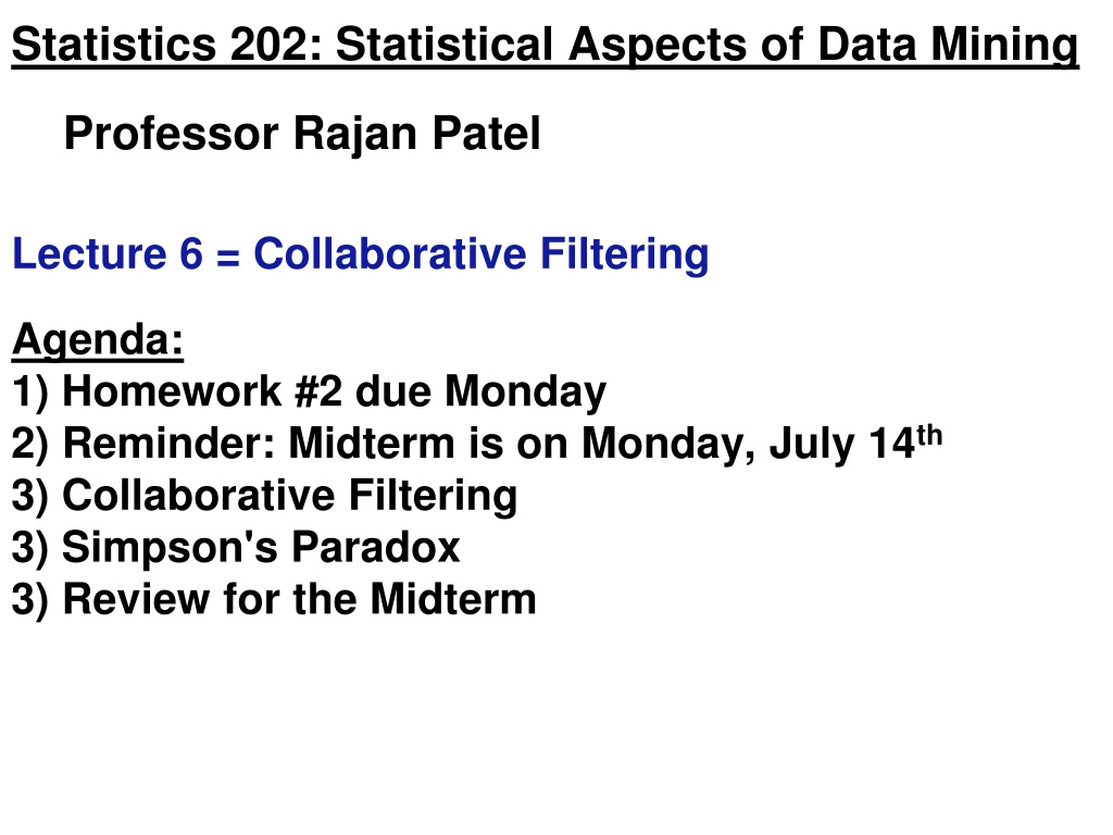
Statistics 202: Statistical Aspects of Data Mining Professor Rajan Patel Lecture 6 = Collaborative Filtering Agenda: 1) Homework #2 due Monday 2) Reminder: Midterm is on Monday, July 14th 3) Collaborative Filtering 3) Simpson's Paradox 3) Review for the Midterm
Announcement Midterm Exam: The midterm exam will be Monday, July 14 Stanford and SCPD students should try to take it in class (4:15 PM) Remote students who can t come to class should take it with a proctor and return it via Scoryst by July 15 at 11:59 PM. You are allowed one 8.5 x 11 inch sheet (front and back) containing notes No books or computers are allowed, but please bring a hand held calculator * The exam will cover the material that we covered in class from Chapters 1,2,3 and 6
The Netflix Prize 100M ratings of movies 18k movies and 48k users On average ~ 5600 ratings / movie On average ~ 208 ratings / user Data collected over several years Ratings are integers from 1 to 5
Objective Reduce RMSE on new data by 10% Current is 0.951, so reduce to 0.856. New data may not have the same distributions as older data (Netflix is growing, more users and movies, fewer movies rated per user and per movie)
A baseline model bui= + bu+ bi Where is the item rating biis the mean rating for that item buis the mean rating for that user Models how critical a user is and how good a movie is, on average.
Collaborative Filtering CF produces recommendations of items based on patterns of ratings or usage (e.g. purchases) without the need for exogenous information about the item or user Relates two fundamentally different entities: items and users
Collaborative Filtering Two main techniques Neighborhood approach Latent factor models Neighborhood methods focus on relationships between items (or users), modeling the preference of a user to an item based on ratings of similar items by that user.
Neighborhood approaches Two items are more similar if a user rated both items similarly. Cluster items based on similarity Or build a kNN based predictive model
Latent factor models Transform items and users to the same latent factor space. Explains ratings by characterizing products and users on factors inferred from user feedback. This new space might identify factors relating to comedy , romance , or a particular actor, etc.
Latent factor models Map items and users into a latent factor space of dimensionality, f
Latent factor models Estimate the parameters with the least squared error with some regularization is a regularization parameter to bias parameters towards 0. Estimate with gradient ascent
Latent factor models Bonus - include information about whether a result was rated at all Each item associated with a new factor vector y which is then used to modify our user features based on which items they rated
Simpsons Paradox (page 384) Occurs when the relationship between a pair of variables across different groups changes when the groups are combined Baseball Example: Batting averages of David Justice and Derek Jeter in 1995 and 1996 1995 1996 Combined Derek Jeter 12/48 .250 183/582 .314 195/630 .310 David Justice 104/411 45/140 149/551 .270 .253 .321 Justice has a better batting average in 1995 and 1996, but overall for the two seasons, he has a lower average
Another example of Simpsons Paradox Real example from a medical study comparing the effectiveness of a treatment on kidney stones Overall success rate Treatment A Treatment B 78% (273/350) 83% (289/350) Above table seems to suggest that Treatment B is more effective, but if we break down the data by kidney stone size, we see that the opposite may be true Treatment A Treatment B 87% (234/270) Small Stones 93% (81/87) 69% (55/80) Large Stones 73% (192/263) 78% (273/350) Both 83% (289/350)
Sample Midterm Question #1: What is the definition of data mining used in your textbook? A) the process of automatically discovering useful information in large data repositories B) the computer-assisted process of digging through and analyzing enormous sets of data and then extracting the meaning of the data C) an analytic process designed to explore data in search of consistent patterns and/or systematic relationships between variables, and then to validate the findings by applying the detected patterns to new subsets of data
Sample Midterm Question #2: If height is measured as short, medium or tall then it is what kind of attribute? A) Nominal B) Ordinal C) Interval D) Ratio
Sample Midterm Question #3: If my data frame in R is called data , which of the following will give me the third column? A) data[2,] B) data[3,] C) data[,2] D) data[,3] E) data(2,) F) data(3,) G) data(,2) H) data(,3)
Sample Midterm Question #4: Compute the confidence for the association rule {b, d} {a} by treating each row as a market basket. Also, state what this value means in plain English.
Sample Midterm Question #5: Compute the standard deviation for the numbers 23, 25, 30. Show your work below.


")