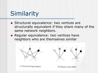
Understanding Similarity and Dissimilarity Measures in Data Mining

Similarity and dissimilarity measures play a crucial role in various data mining techniques like clustering, nearest neighbor classification, and anomaly detection. These measures help quantify how alike or different data objects are, facilitating efficient data analysis and decision-making processes. Proximity measures and transformations are utilized to convert similarities to dissimilarities or vice versa, ensuring compatibility with different algorithms and software packages.

Download Presentation

Please find below an Image/Link to download the presentation.
The content on the website is provided AS IS for your information and personal use only. It may not be sold, licensed, or shared on other websites without obtaining consent from the author. Download presentation by click this link. If you encounter any issues during the download, it is possible that the publisher has removed the file from their server.
E N D
Presentation Transcript
Data Mining Prof. Dr. Nizamettin AYDIN naydin@yildiz.edu.tr http://www3.yildiz.edu.tr/~naydin 1
Data Mining Similarity and Dissimilarity Measures Outline Similarity and Dissimilarity between Simple Attributes Dissimilarities between Data Objects Similarities between Data Objects Examples of Proximity Mutual Information Issues in Proximity Selecting the Right Proximity Measure 2
Similarity and Dissimilarity Measures Similarity and dissimilarity are important because they are used by a number of data mining techniques, such as clustering, nearest neighbor classification, and anomaly detection. In many cases, the initial data set is not needed once these similarities or dissimilarities have been computed. Such approaches can be viewed as transforming the data to a similarity (dissimilarity) space and then performing the analysis. 3
Similarity and Dissimilarity Measures Similarity measure Numerical measure of how alike two data objects are. Is higher when objects are more alike. Often falls in the range [0,1] Dissimilarity measure Numerical measure of how different two data objects are Lower when objects are more alike Minimum dissimilarity is often 0, upper limit varies The term distance is used as a synonym for dissimilarity Proximity refers to a similarity or dissimilarity 4
Transformations often applied to convert a similarity to a dissimilarity, or vice versa, or to transform a proximity measure to fall within a particular range, such as [0,1]. For instance, we may have similarities that range from 1 to 10, but the particular algorithm or software package that we want to use may be designed to work only with dissimilarities, or it may work only with similarities in the interval [0,1] Frequently, proximity measures, especially similarities, are defined or transformed to have values in the interval [0,1]. 5
Transformations often applied to convert a similarity to a dissimilarity, or vice versa, or to transform a proximity measure to fall within a particular range, such as [0,1]. For instance, we may have similarities that range from 1 to 10, but the particular algorithm or software package that we want to use may be designed to work only with dissimilarities, or it may work only with similarities in the interval [0,1] Frequently, proximity measures, especially similarities, are defined or transformed to have values in the interval [0,1]. 6
Transformations Example: If the similarities between objects range from 1 (not at all similar) to 10 (completely similar), we can make them fall within the range [0, 1] by using the transformation s =(s-1)/9,where s and s are the original and new similarity values, respectively. The transformation of similarities and dissimilarities to the interval [0, 1] s =(s-smin)/(smax- smin),where smaxand sminare the maximum and minimum similarity values. d =(d-dmin)/(dmax- dmin),where dmaxand dminare the maximum and minimum dissimilarity values. 7
Transformations However, there can be complications in mapping proximity measures to the interval [0, 1] using a linear transformation. If, for example, the proximity measure originally takes values in the interval [0, ], then dmaxis not defined and a nonlinear transformation is needed. Values will not have the same relationship to one another on the new scale. Consider the transformation d=d/(1+d) for a dissimilarity measure that ranges from 0 to . Given dissimilarities 0, 0.5, 2, 10, 100, 1000 Transformed dissimilarities 0, 0.33, 0.67, 0.90, 0.99, 0.999. Larger values on the original dissimilarity scale are compressed into the range of values near 1, but whether this is desirable depends on the application. 8
Similarity/Dissimilarity for Simple Attributes The following table shows the similarity and dissimilarity between two objects, x and y, with respect to a single, simple attribute. Next, we consider more complicated measures of proximity between objects that involve multiple attributes: dissimilarities between data objects similarities between data objects. 9
Distances - Euclidean Distance The Euclidean distance, d , between two points, x and y , in one-, two-, three-, or higher- dimensional space, is given by where n is the number of dimensions (attributes) and xkand ykare, respectively, the kthattributes (components) of data objects x and y. Standardization is necessary, if scales differ. 10
Distances - Euclidean Distance 3 point p1 p2 p3 p4 x 0 2 3 5 y 2 0 1 1 p1 2 p3 p4 1 p2 0 0 1 2 3 4 5 6 p1 p2 2.828 p3 3.162 1.414 p4 5.099 3.162 p1 p2 p3 p4 0 2.828 3.162 5.099 0 1.414 3.162 0 2 2 0 11
Distances - Minkowski Distance Minkowski Distance is a generalization of Euclidean Distance, and is given by where r is a parameter, n is the number of dimensions (attributes) and xkand ykare are, respectively, the kth attributes (components) of data objects x and y. 12
Distances - Minkowski Distance The following are the three most common examples of Minkowski distances. r = 1 , City block (Manhattan, taxicab, L1norm) distance. A common example of this for binary vectors is the Hamming distance, which is just the number of bits that are different between two binary vectors r = 2 , Euclidean distance (L2norm) r = , Supremum (Lmaxnorm, L norm) distance. This is the maximum difference between any component of the vectors Do not confuse r with n, i.e., all these distances are defined for all numbers of dimensions. 13
Distances - Minkowski Distance 3 L1 p1 p2 p3 p4 p1 0 4 4 6 p2 4 0 2 4 p3 4 2 0 2 p4 6 4 2 0 p1 2 p3 p4 1 p2 0 L2 p1 p2 p3 p4 p1 p2 2.828 p3 3.162 1.414 p4 5.099 3.162 0 1 2 3 4 5 6 0 2.828 3.162 5.099 0 point p1 p2 p3 p4 x 0 2 3 5 y 2 0 1 1 1.414 3.162 0 2 2 0 p1 p2 p3 p4 L p1 p2 p3 p4 0 2 3 5 2 0 1 3 3 1 0 2 5 3 2 0 Distance Matrix 14
Distances - Mahalanobis Distance Mahalonobis distance is the distance between a point and a distribution (not between two distinct points). It is effectively a multivariate equivalent of the Euclidean distance. It transforms the columns into uncorrelated variables Scale the columns to make their variance equal to 1 Finally, it calculates the Euclidean distance. It is defined as where 1is the inverse of the covariance matrix of the data. 15
Distances - Mahalanobis Distance In the Figure, there are 1000 points, whose x and y attributes have a correlation of 0.6. The Euclidean distance between the two large points at the opposite ends of the long axis of the ellipse is 14.7, but Mahalanobis distance is only 6. This is because the Mahalanobis distance gives less emphasis to the direction of largest variance. 16
Distances - Mahalanobis Distance Covariance Matrix: = 2 . 0 3 . 0 2 . 0 3 . 0 A: (0.5, 0.5) C B: (0, 1) B A C: (1.5, 1.5) Mahal(A,B) = 5 Mahal(A,C) = 4 17
Common Properties of a Distance Distances, such as the Euclidean distance, have some well-known properties. If d(x, y) is the distance between two points, x and y, then the following properties hold. Positivity d(x, y) 0 for all x and y d(x, y) = 0 only if x = y Symmetry d(x, y) = d(y, x) for all x and y Triangle Inequality d(x, z) d(x, y) + d(y, z) for all points x, y, and z Measures that satisfy all three properties are known as metrics 18
Common Properties of a Similarity If s(x, y) is the similarity between points x and y, then the typical properties of similarities are the following: Positivity s(x, y) = 1 only if x = y. (0 s 1) Symmetry s(x, y) = s(y, x) for all x and y For similarities, the triangle inequality typically does not hold However, a similarity measure can be converted to a metric distance 19
A Non-symmetric Similarity Measure Example Consider an experiment in which people are asked to classify a small set of characters as they flash on a screen. The confusion matrix for this experiment records how often each character is classified as itself, and how often each is classified as another character. Using the confusion matrix, we can define a similarity measure between a character x and a character y as the number of times that x is misclassified as y, but note that this measure is not symmetric. 20
A Non-symmetric Similarity Measure Example For example, suppose that 0 appeared 200 times and was classified as a 0 160 times, but as an o 40 times. Likewise, suppose that o appeared 200 times and was classified as an o 170 times, but as 0 only 30 times. Then, s(0,o) = 40, but s(o, 0) = 30. In such situations, the similarity measure can be made symmetric by setting s (x, y) = s (y, x) = (s(x, y)+s(y, x))/2, where s indicates the new similarity measure. 21
Similarity Measures for Binary Data Similarity measures between objects that contain only binary attributes are called similarity coefficients, and typically have values between 0 and 1. Let x and y be two objects that consist of n binary attributes. The comparison of two binary vectors, leads to the following quantities (frequencies): f00= the number of attributes where x is 0 and y is 0 f01= the number of attributes where x is 0 and y is 1 f10= the number of attributes where x is 1 and y is 0 f11= the number of attributes where x is 1 and y is 1 22
Similarity Measures for Binary Data Simple Matching Coefficient (SMC) One commonly used similarity coefficient This measure counts both presences and absences equally. Consequently, the SMC could be used to find students who had answered questions similarly on a test that consisted only of true/false questions. 23
Similarity Measures for Binary Data Jaccard Similarity Coefficient frequently used to handle objects consisting of asymmetric binary attributes This measure counts both presences and absences equally. Consequently, the SMC could be used to find students who had answered questions similarly on a test that consisted only of true/false questions. 24
SMC versus Jaccard: Example Calculate SMC and J for the binary vectors, x = (1 0 0 0 0 0 0 0 0 0) y = (0 0 0 0 0 0 1 0 0 1) f01= 2 (the number of attributes where x was 0 and y was 1) f10= 1 (the number of attributes where x was 1 and y was 0) f00= 7 (the number of attributes where x was 0 and y was 0) f11= 0 (the number of attributes where x was 1 and y was 1) SMC = (f11+ f00) / (f01+ f10+ f11+ f00) = (0 + 7) / (2 + 1 + 0 + 7) J = (f11) / (f01+ f10+ f11) = 0 / (2 + 1 + 0) = 0.7 = 0 25
Cosine Similarity Cosine Similarity is one of the most common measures of document similarity If x and y are two document vectors, then where indicates vector or matrix transpose and x,y indicates the inner product of the two vectors, and ? is the length of vector x, 26
Cosine Similarity Cosine similarity really is a measure of the (cosine of the) angle between x and y. Thus, if the cosine similarity is 1, the angle between x and y is 0 , and x and y are the same except for length. If the cosine similarity is 0, then the angle between x and y is 90 , and they do not share any terms (words). It can also be written as 27
Cosine Similarity - Example Cosine Similarity between two document vectors This example calculates the cosine similarity for the following two data objects, which might represent document vectors: x = (3, 2, 0, 5, 0, 0, 0, 2, 0, 0) y = (1, 0, 0, 0, 0, 0, 0, 1, 0, 2) x,y = 3 1 + 2 0 + 0 0 + 5 0 + 0 0 + 0 0 + 0 0 + 2 1 + 0 0 + 0 2 = 5 32+ 22+ 02+ 52+ 02+ 02+ 02+ 22+ 02+ 02= 6.48 ? = 12+ 02+ 02+ 02+ 02+ 02+ 02+ 12+ 02+ 22= 2.45 x,y ? ?= ? = 5 cos x,y = 6.48 2.45= 0.31 28
Extended Jaccard Coefficient Also known as Tanimoto Coefficient The extended Jaccard coefficient can be used for document data and that reduces to the Jaccard coefficient in the case of binary attributes. This coefficient, which we shall represent as EJ, is defined by the following equation: 29
Correlation used to measure the linear relationship between two sets of values that are observed together. Thus, correlation can measure the relationship between two variables (height and weight) or between two objects (a pair of temperature time series). Correlation is used much more frequently to measure the similarity between attributes since the values in two data objects come from different attributes, which can have very different attribute types and scales. There are many types of correlation 30
Correlation - Pearsons correlation between two sets of numerical values, i.e., two vectors, x and y, is defined by: where the following standard statistical notation and definitions are used: 31
Correlation Example (Perfect Correlation) Correlation is always in the range 1 to 1. A correlation of 1 ( 1) means that x and y have a perfect positive (negative) linear relationship; that is, xk= ayk+ b, where a and b are constants. The following two vectors x and y illustrate cases where the correlation is 1 and +1, respectively. x = ( 3, 6, 0, 3, 6) y = ( 1, 2, 0, 1, 2) x = (3, 6, 0, 3, 6) y = (1, 2, 0, 1, 2) corr(x, y) = 1 xk= 3yk corr(x, y) = 1 xk= 3yk 32
Correlation Example (Nonlinear Relationships) If the correlation is 0, then there is no linear relationship between the two sets of values. However, nonlinear relationships can still exist. In the following example, y?= x? 2, but their correlation is 0. x = (-3, -2, -1, 0, 1, 2, 3) y = (9, 4, 1, 0, 1, 4, 9) y?= x? mean(x) = 0, mean(y) = 4 std(x) = 2.16, std(y) = 3.74 ???? =( 3)(5)+( 2)(0)+( 1)( 3)+(0)( 4)+(1)( 3)+(2)(0)+(3)(5) 6 2.16 3.74 2 = 0 33
Visually Evaluating Correlation Scatter plots showing the similarity from 1 to 1. 34
Correlation vs Cosine vs Euclidean Distance Compare the three proximity measures according to their behavior under variable transformation scaling: multiplication by a value translation: adding a constant Property Cosine Correlation Euclidean Distance Invariant to scaling (multiplication) Yes Yes No Invariant to translation (addition) No Yes No Consider the example x = (1, 2, 4, 3, 0, 0, 0), ys= y 2 = (2, 4, 6, 8, 0, 0, 0) y = (1, 2, 3, 4, 0, 0, 0) yt= y + 5 = (6, 7, 8, 9, 5, 5, 5) (x , y) (x , ys) 0.9667 (x , yt) 0.7940 Measure Cosine 0.9667 Correlation 0.9429 0.9429 0.9429 Euclidean Distance 1.4142 5.8310 14.2127 35
Correlation vs cosine vs Euclidean distance Choice of the right proximity measure depends on the domain What is the correct choice of proximity measure for the following situations? Comparing documents using the frequencies of words Documents are considered similar if the word frequencies are similar Comparing the temperature in Celsius of two locations Two locations are considered similar if the temperatures are similar in magnitude Comparing two time series of temperature measured in Celsius Two time series are considered similar if their shape is similar, i.e., they vary in the same way over time, achieving minimums and maximums at similar times, etc. 36
Comparison of Proximity Measures Domain of application Similarity measures tend to be specific to the type of attribute and data Record data, images, graphs, sequences, 3D-protein structure, etc. tend to have different measures However, one can talk about various properties that you would like a proximity measure to have Symmetry is a common one Tolerance to noise and outliers is another Ability to find more types of patterns? Many others possible The measure must be applicable to the data and produce results that agree with domain knowledge 37
Information Based Measures Information theory is a well-developed and fundamental disciple with broad applications Some similarity measures are based on information theory Mutual information in various versions Maximal Information Coefficient (MIC) and related measures General and can handle non-linear relationships Can be complicated and time intensive to compute 38
Information relates to possible outcomes of an event transmission of a message, flip of a coin, or measurement of a piece of data The more certain an outcome, the less information that it contains and vice-versa For example, if a coin has two heads, then an outcome of heads provides no information More quantitatively, the information is related the probability of an outcome The smaller the probability of an outcome, the more information it provides and vice-versa Entropy is the commonly used measure 39
Entropy For a variable (event), X, with n possible values (outcomes), x1, x2 , xn each outcome having probability, p1, p2 , pn the entropy of X , H(X), is given by ? ? ? = ??log2?? ?=1 Entropy is between 0 and log2n and is measured in bits Thus, entropy is a measure of how many bits it takes to represent an observation of X on average 40
Entropy Examples For a coin with probability p of heads and probability q = 1 p of tails ? = ?log2? ?log2? For p= 0.5, q = 0.5 (fair coin) H = 1 For p = 1 or q = 1, H = 0 What is the entropy of a fair four-sided die? 41
Entropy for Sample Data: Example p -plog2p Hair Color Black Brown Blond Red Other Total Count 75 15 5 0 5 100 0.75 0.15 0.05 0.00 0.05 1.0 0.3113 0.4105 0.2161 0 0.2161 1.1540 Maximum entropy is log25 = 2.3219 42
Entropy for Sample Data Suppose we have a number of observations (m) of some attribute, X, e.g., the hair color of students in the class, where there are n different possible values And the number of observation in the ithcategory is mi Then, for this sample ? ?? ?log2 ?? ? ? ? = ?=1 For continuous data, the calculation is harder 43
Mutual Information used as a measure of similarity between two sets of paired values that is sometimes used as an alternative to correlation, particularly when a nonlinear relationship is suspected between the pairs of values. This measure comes from information theory, which is the study of how to formally define and quantify information. It is a measure of how much information one set of values provides about another, given that the values come in pairs, e.g., height and weight. If the two sets of values are independent, i.e., the value of one tells us nothing about the other, then their mutual information is 0. 44
Mutual Information Information one variable provides about another Formally, ? ?,? = ? ? + ? ? ?(?,?), where H(X,Y) is the joint entropy of X and Y, ? ?,? = ???log2??? ? ? where pijis the probability that the ithvalue of X and the jthvalue of Y occur together For discrete variables, this is easy to compute Maximum mutual information for discrete variables is log2(min( nX, nY), where nX(nY) is the number of values of X (Y) 45
Mutual Information Example Evaluating Nonlinear Relationships with Mutual Information Recall Example where y?= x? x = ( 3, 2, 1, 0, 1, 2, 3) I(x, y) = H(x) + H(y) H(x, y) = 1.9502 Entropy for y 2, but their correlation was 0. y = ( 9, 4, 1, 0, 1, 4, 9) Joint entropy for x and y Entropy for x 46
Mutual Information Example p -plog2p p -plog2p Student Status Count Student Status Grade Count Undergrad 45 0.45 0.5184 Undergrad A 5 0.05 0.2161 Grad 55 0.55 0.4744 Undergrad B 30 0.30 0.5211 Total 100 1.00 0.9928 Undergrad C 10 0.10 0.3322 p -plog2p 0.5301 Grade Count Grad A 30 0.30 0.5211 A 35 0.35 Grad B 20 0.20 0.4644 B 50 0.50 0.5000 Grad C 5 0.05 0.2161 C 15 0.15 0.4105 Total 100 1.00 2.2710 Total 100 1.00 1.4406 Mutual information of Student Status and Grade = 0.9928 + 1.4406 - 2.2710 = 0.1624 47
Maximal Information Coefficient Applies mutual information to two continuous variables Consider the possible binnings of the variables into discrete categories nX nY N0.6where nXis the number of values of X nYis the number of values of Y N is the number of samples (observations, data objects) Compute the mutual information Normalized by log2(min( nX, nY) Take the highest value Reshef, David N., Yakir A. Reshef, Hilary K. Finucane, Sharon R. Grossman, Gilean McVean, Peter J. Turnbaugh, Eric S. Lander, Michael Mitzenmacher, and Pardis C. Sabeti. "Detecting novel associations in large data sets." science 334, no. 6062 (2011): 1518-1524. 48
General Approach for Combining Similarities Sometimes attributes are of many different types, but an overall similarity is needed. For the kthattribute, compute a similarity, sk(x, y), in the range [0, 1]. Define an indicator variable, k, for the kthattribute as follows: k= 0 if the kthattribute is an asymmetric attribute and both objects have a value of 0, or if one of the objects has a missing value for the kth attribute k= 1 otherwise Compute 49
Using Weights to Combine Similarities May not want to treat all attributes the same. Use non-negative weights ?? ? ?=1 ??????(?,?) ?=1 ???? ?????????? ?,? = ? Can also define a weighted form of distance 50


")
")