Introduction to Frequent Itemsets and Association Rules in Data Mining

The birth of Data Mining is credited to papers by Agrawal, Imielinski, and Swami in the early 1990s, focusing on Association Rules and Frequent Itemsets. Market-Basket data analysis involves finding common item combinations, with applications in retail strategies and web content analysis.

Download Presentation

Please find below an Image/Link to download the presentation.
The content on the website is provided AS IS for your information and personal use only. It may not be sold, licensed, or shared on other websites without obtaining consent from the author. Download presentation by click this link. If you encounter any issues during the download, it is possible that the publisher has removed the file from their server.
E N D
Presentation Transcript
DATA MINING LECTURE 3 Frequent Itemsets Association Rules
This is how it all started Rakesh Agrawal, Tomasz Imielinski, Arun N. Swami: Mining Association Rules between Sets of Items in Large Databases. SIGMOD Conference 1993: 207- 216 Rakesh Agrawal, Ramakrishnan Srikant: Fast Algorithms for Mining Association Rules in Large Databases. VLDB 1994: 487-499 These two papers are credited with the birth of Data Mining For a long time people were fascinated with Association Rules and Frequent Itemsets Some people (in industry and academia) still are.
3 Market-Basket Data A large set of items, e.g., things sold in a supermarket. A large set of baskets, each of which is a small set of the items, e.g., the things one customer buys on one day.
4 Market-Baskets (2) Really, a general many-to-many mapping (association) between two kinds of things, where the one (the baskets) is a set of the other (the items) But we ask about connections among items, not baskets. The technology focuses on common events, not rare events ( long tail ).
Frequent Itemsets Given a set of transactions, find combinations of items (itemsets) that occur frequently Support ? ? : number of transactions that contain itemset I Market-Basket transactions Items: {Bread, Milk, Diaper, Beer, Eggs, Coke} TID 1 2 3 4 5 Items Bread, Milk Bread, Diaper, Beer, Eggs Milk, Diaper, Beer, Coke Bread, Milk, Diaper, Beer Bread, Milk, Diaper, Coke Examples of frequent itemsets ? ? 3 {Bread}: 4 {Milk} : 4 {Diaper} : 4 {Beer}: 3 {Diaper, Beer} : 3 {Milk, Bread} : 3
6 Applications (1) Items = products; baskets = sets of products someone bought in one trip to the store. Example application: given that many people buy beer and diapers together: Run a sale on diapers; raise price of beer. Only useful if many buy diapers & beer.
7 Applications (2) Baskets = Web pages; items = words. Example application: Unusual words appearing together in a large number of documents, e.g., Brad and Angelina, may indicate an interesting relationship.
8 Applications (3) Baskets = sentences; items = documents containing those sentences. Example application: Items that appear together too often could represent plagiarism. Notice items do not have to be in baskets.
Definition: Frequent Itemset Itemset A collection of one or more items Example: {Milk, Bread, Diaper} k-itemset An itemset that contains k items Support ( ) Count: Frequency of occurrence of an itemset E.g. ({Milk, Bread,Diaper}) = 2 Fraction: Fraction of transactions that contain an itemset E.g. s({Milk, Bread, Diaper}) = 40% Frequent Itemset An itemset whose support is greater than or equal to a minsup threshold TID 1 2 3 4 5 Items Bread, Milk Bread, Diaper, Beer, Eggs Milk, Diaper, Beer, Coke Bread, Milk, Diaper, Beer Bread, Milk, Diaper, Coke ? ? minsup
Mining Frequent Itemsets task Input: A set of transactions T, over a set of items I Output: All itemsets with items in I having support minsup threshold Problem parameters: N = |T|: number of transactions d = |I|: number of (distinct) items w: max width of a transaction Number of possible itemsets? M = 2d Scale of the problem: WalMart sells 100,000 items and can store billions of baskets. The Web has billions of words and many billions of pages.
The itemset lattice null A B C D E AB AC AD AE BC BD BE CD CE DE ABC ABD ABE ACD ACE ADE BCD BCE BDE CDE ABCD ABCE ABDE ACDE BCDE Given d items, there are 2d possible itemsets ABCDE
A Nave Algorithm Brute-force approach, each itemset is a candidate : Consider each itemset in the lattice, and count the support of each candidate by scanning the data Time Complexity ~ O(NMw) , Space Complexity ~ O(M) OR Scan the data, and for each transaction generate all possible itemsets. Keep a count for each itemset in the data. Time Complexity ~ O(N2w) , Space Complexity ~ O(M) Expensive since M = 2d !!! List of Candidates Transactions TID Items 1 2 3 4 5 Bread, Milk Bread, Diaper, Beer, Eggs Milk, Diaper, Beer, Coke Bread, Milk, Diaper, Beer Bread, Milk, Diaper, Coke w M N
13 Computation Model Typically, data is kept in flat files rather than in a database system. Stored on disk. Stored basket-by-basket. Expand baskets into pairs, triples, etc. as you read baskets. Use k nested loops to generate all sets of size k.
Example file: retail 0 1 2 3 4 5 6 7 8 9 10 11 12 13 14 15 16 17 18 19 20 21 22 23 24 25 26 27 28 29 30 31 32 33 34 35 36 37 38 39 40 41 42 43 44 45 46 38 39 47 48 38 39 48 49 50 51 52 53 54 55 56 57 58 32 41 59 60 61 62 3 39 48 63 64 65 66 67 68 32 69 48 70 71 72 39 73 74 75 76 77 78 79 36 38 39 41 48 79 80 81 82 83 84 41 85 86 87 88 39 48 89 90 91 92 93 94 95 96 97 98 99 100 101 36 38 39 48 89 39 41 102 103 104 105 106 107 108 38 39 41 109 110 39 111 112 113 114 115 116 117 118 119 120 121 122 123 124 125 126 127 128 129 130 131 132 133 48 134 135 136 39 48 137 138 139 140 141 142 143 144 145 146 147 148 149 39 150 151 152 38 39 56 153 154 155 Example: items are positive integers, and each basket corresponds to a line in the file of space separated integers
15 Computation Model (2) The true cost of mining disk-resident data is usually the number of disk I/O s. In practice, association-rule algorithms read the data in passes all baskets read in turn. Thus, we measure the cost by the number of passes an algorithm takes.
16 Main-Memory Bottleneck For many frequent-itemset algorithms, main memory is the critical resource. As we read baskets, we need to count something, e.g., occurrences of pairs. The number of different things we can count is limited by main memory. Swapping counts in/out is a disaster (why?).
The Apriori Principle Apriori principle (Main observation): If an itemset is frequent, then all of its subsets must also be frequent If an itemset is not frequent, then all of its supersets cannot be frequent ) ( : , Y X Y X ( ) ( ) s X s Y The support of an itemset never exceeds the support of its subsets This is known as the anti-monotone property of support
Illustration of the Apriori principle Frequent subsets Found to be frequent
Illustration of the Apriori principle null null A A B B C C D D E E AB AB AC AC AD AD AE AE BC BC BD BD BE BE CD CD CE CE DE DE Found to be Infrequent ABC ABC ABD ABD ABE ABE ACD ACD ACE ACE ADE ADE BCD BCD BCE BCE BDE BDE CDE CDE ABCD ABCD ABCE ABCE ABDE ABDE ACDE ACDE BCDE BCDE Infrequent supersets ABCDE ABCDE Pruned
The Apriori algorithm Ck = candidate itemsets of size k Lk = frequent itemsets of size k Level-wise approach 1. k = 1, C1 = all items 2. While Ck not empty 3. Scan the database to find which itemsets in Ck are frequent and put them into Lk 4. Use Lkto generate a collection of candidate itemsets Ck+1 of size k+1 5. k = k+1 Frequent itemset generation Candidate generation R. Agrawal, R. Srikant: "Fast Algorithms for Mining Association Rules", Proc. of the 20th Int'l Conference on Very Large Databases, 1994.
Illustration of the Apriori principle TID 1 2 3 4 5 Items Bread, Milk Bread, Diaper, Beer, Eggs Milk, Diaper, Beer, Coke Bread, Milk, Diaper, Beer Bread, Milk, Diaper, Coke minsup = 3 Items (1-itemsets) Item Bread Coke Milk Beer Diaper Eggs Count 4 2 4 3 4 1 Pairs (2-itemsets) Itemset {Bread,Milk} {Bread,Beer} {Bread,Diaper} {Milk,Beer} {Milk,Diaper} {Beer,Diaper} Count 3 2 3 2 3 3 (No need to generate candidates involving Coke or Eggs) Triplets (3-itemsets) If every subset is considered, 6 1 + 6 With support-based pruning, 6 1 + 4 Itemset {Bread,Milk,Diaper} Only this triplet has all subsets to be frequent But it is below the minsup threshold Count 2 2 + 6 3 = 6 + 15 + 20 = 41 2 + 1 = 6 + 6 + 1 = 13
Candidate Generation Basic principle (Apriori): An itemset of size k+1 is candidate to be frequent only if all of its subsets of size k are known to be frequent Main idea: Construct a candidate of size k+1 by combining frequent itemsets of size k If k = 1, take the all pairs of frequent items If k > 1, join pairs of itemsets that differ by just one item For each generated candidate itemset ensure that all subsets of size k are frequent.
23 A-Priori for All Frequent Itemsets One pass for each k. Needs room in main memory to count each candidate k -set. For typical market-basket data and reasonable support (e.g., 1%), k = 2 requires the most memory.
24 Picture of A-Priori Frequent items Item counts Counts of pairs of frequent items Pass 1 Pass 2
25 Details of Main-Memory Counting Two approaches: 1. Count all pairs, using a triangular matrix = one dimensional array that stores the lower diagonal. 2. Keep a table of triples [i, j, c] = the count of the pair of items {i, j } is c. (1) requires only 4 bytes/pair. Note: always assume integers are 4 bytes. (2) requires 12 bytes, but only for those pairs with count > 0.
Factors Affecting Complexity Choice of minimum support threshold lowering support threshold results in more frequent itemsets this may increase number of candidates and max length of frequent itemsets Dimensionality (number of items) of the data set more space is needed to store support count of each item if number of frequent items also increases, both computation and I/O costs may also increase Size of database since Apriori makes multiple passes, run time of algorithm may increase with number of transactions Average transaction width transaction width increases with denser data sets This may increase max length of frequent itemsets and traversals of hash tree (number of subsets in a transaction increases with its width)
Association Rule Mining Given a set of transactions, find rules that will predict the occurrence of an item based on the occurrences of other items in the transaction Market-Basket transactions Example of Association Rules TID 1 2 3 4 5 Items Bread, Milk Bread, Diaper, Beer, Eggs Milk, Diaper, Beer, Coke Bread, Milk, Diaper, Beer Bread, Milk, Diaper, Coke {Diaper} {Beer}, {Milk, Bread} {Eggs,Coke}, {Beer, Bread} {Milk}, Implication means co-occurrence, not causality!
Definition: Association Rule Association Rule An implication expression of the form X Y, where X and Y are itemsets Example: {Milk, Diaper} {Beer} Rule Evaluation Metrics Support (s) TID 1 2 3 4 5 Items Bread, Milk Bread, Diaper, Beer, Eggs Milk, Diaper, Beer, Coke Bread, Milk, Diaper, Beer Bread, Milk, Diaper, Coke Fraction of transactions that contain both X and Y Example: Milk { , Diaper } Beer the probability P(X,Y) that X and Y occur together Confidence (c) = ( Milk , Diaper, Beer ) 2 = = 4 . 0 s | T | 5 Measures how often items in Y appear in transactions that contain X ( Milk, Diaper, Beer ) 2 = = = . 0 67 c ( Milk , Diaper ) 3 the conditional probability P(Y|X) that Y occurs given that X has occurred.
Association Rule Mining Task Input: A set of transactions T, over a set of items I Output: All rules with items in I having support minsup threshold confidence minconf threshold
Mining Association Rules Two-step approach: 1. Frequent Itemset Generation Generate all itemsets whose support minsup 2. Rule Generation Generate high confidence rules from each frequent itemset, where each rule is a partitioning of a frequent itemset into Left-Hand-Side (LHS) and Right-Hand-Side (RHS) Frequent itemset: {A,B,C,D} Rule: AB CD
Rule Generation We have all frequent itemsets, how do we get the rules? For every frequent itemset S, we find rules of the form L S L , where L S, that satisfy the minimum confidence requirement Example: L = {A,B,C,D} Candidate rules: A BCD, B ACD, C ABD, D ABC AB CD, AC BD, AD BC, BD AC, CD AB, ABC D, BCD A, If |L| = k, then there are 2k 2 candidate association rules (ignoring L and L) BC AD,
Rule Generation How to efficiently generate rules from frequent itemsets? In general, confidence does not have an anti-monotone property c(ABC D) can be larger or smaller than c(AB D) But confidence of rules generated from the same itemset has an anti-monotone property e.g., L = {A,B,C,D}: c(ABC D) c(AB CD) c(A BCD) Confidence is anti-monotone w.r.t. number of items on the RHS of the rule
Rule Generation for Apriori Algorithm ABCD=>{ } ABCD=>{ } Low Confidence Rule BCD=>A BCD=>A ACD=>B ACD=>B ABD=>C ABD=>C ABC=>D ABC=>D CD=>AB CD=>AB BD=>AC BD=>AC BC=>AD BC=>AD AD=>BC AD=>BC AC=>BD AC=>BD AB=>CD AB=>CD D=>ABC D=>ABC C=>ABD C=>ABD B=>ACD B=>ACD A=>BCD A=>BCD Pruned Rules Lattice of rules created by the RHS
Rule Generation for APriori Algorithm Candidate rule is generated by merging two rules that share the same prefix in the RHS CD->AB BD->AC join(CD AB,BD AC) would produce the candidate rule D ABC Prune rule D ABC if its subset AD BC does not have high confidence D->ABC Essentially we are doing APriori on the RHS
Diskusi 1. Explorasi mengenai Na ve Algorithm dan Apriori Algorithm. Berdasarkan hasil explorasi anda, bagaimana karakteristik na ve algorithm dan apriori algorithm. Bagaimana pemanfaatan kedua algoritma tersebut dalam data mining 2. Cari tahu mengenai Rule Prune. Untuk apa rule prune di implementasikan? 3. Apa yang dimaksud dengan Association rule. Di dunia nyata apa manfaat association rule. Beri contoh.