Improved Rectangular Matrix Multiplication Using Coppersmith-Winograd Tensor

In this research, the complexity of rectangular matrix multiplication is enhanced by analyzing the fourth power of the Coppersmith-Winograd tensor. By extending the understanding of the tensor's power, significant advancements have been made in the efficiency of non-square matrix multiplication, surpassing previous algorithms based on the second power.

Download Presentation

Please find below an Image/Link to download the presentation.
The content on the website is provided AS IS for your information and personal use only. It may not be sold, licensed, or shared on other websites without obtaining consent from the author. Download presentation by click this link. If you encounter any issues during the download, it is possible that the publisher has removed the file from their server.
E N D
Presentation Transcript
Improved Rectangular Matrix Multiplication using Powers of the Coppersmith-Winograd Tensor Fran ois Le Gall Kyoto University Florent Urrutia IRIF, Universit Paris Diderot WACT 2018
Overview of the Result Improvements of the complexity of square matrix multiplication have been obtained in the past few years by analyzing powers of a construction called the Coppersmith-Winograd tensor The best known algorithms for rectangular (non-square) matrix multiplication are based on the second power of the Coppersmith-Winograd tensor Our result We improve the complexity of rectangular (non-square) matrix multiplication by analyzing the fourth power of the Coppersmith-Winograd tensor
Square Matrix Multiplication Compute the product of two n x n matrices A and B over a field n = n cij n aij bij n n n n multiplications and (n-1) additions ? for all 1 i n and 1 j n cij= aikbkj ?=1 One of the most fundamental problems in mathematics and computer science Trivial algorithm:n2(2n-1)=O(n3)arithmetic operations
Exponent of Square Matrix Multiplication Compute the product of two n x n matrices A and B over a field Exponent of square matrix multiplication this product can be computed using arithmetic operations ? ?? = inf ? the product can be computed using O(n + ) arithmetic operations for any >0 trivial algorithm: O(n3) arithmetic operations 3 trivial lower bound: 2
History of the main improvements on the exponent of square matrix multiplication Upper bound 3 < 2.81 1969 Strassen < 2.79 1979 Pan < 2.78 1979 Bini, Capovani, Romani and Lotti < 2.55 1981 Sch nhage < 2.53 1981 Pan < 2.52 1982 Romani < 2.50 1982 Coppersmith and Winograd < 2.48 1986 Strassen < 2.376 1987 Coppersmith and Winograd < 2.373 2010~2014 Stothers, Vassilevska Williams, LG Year Authors Some of these bounds have been recovered using a group theoretic approach [Cohn, Umans 2003] [Cohn, Kleinberg, Szegedy, Umans 2005] [Cohn, Umans 2013]
How are these upper bounds obtained? Find a basic construction (of constant size) with small arithmetic complexity tensor small rank Apply some generic technique to derive an upper bound on Example 1: < 2.81 [Strassen 1969] basic construction: the product of two 2 x 2 matrices can be computed with only 7 multiplications generic technique: recursion two n x n matrices can be multiplied with O(n2.81) operations Example 2: < 2.55 [Sch nhage 1981] basic construction: the direct sum of two small matrix products generic technique: the asymptotic sum inequality Example 3: < 2.388 [Coppersmith and Winograd 1987] basic construction: the Coppersmith-Winograd tensor (CW tensor) generic technique: the laser method
How are these upper bounds obtained? Find a basic construction (of constant size) with small arithmetic complexity tensor small rank Apply some generic technique to derive an upper bound on Example 4: < 2.376 [Coppersmith and Winograd 1987] basic construction: generic technique: the laser method the second tensor power of the CW tensor 2= ?CW ?CW ?CW Example 3: < 2.388 [Coppersmith and Winograd 1987] basic construction: the Coppersmith-Winograd tensor (CW tensor) generic technique: the laser method ?CW
Higher powers of the CW tensor Analyzing ?CWby the laser method gives < 2.388 Analyzing ?CW 2by the laser method gives < 2.376 What about higher powers? Analyzing the third power was explicitly mentioned as an open problem by Coppersmith and Winograd in 1990 The third power does not (seem to) give any improvement But higher powers actually do!
Higher powers of the CW tensor ?by the laser method Upper bounds on obtained by analyzing ?CW m Upper bound Authors < 2.3871900 1 Coppersmith and Winograd (1987) < 2.3754770 2 Coppersmith and Winograd (1987) < 2.3729269 < 2.3729 < 2.3728640 < 2.3728639 4 Stothers (2010), Vassilevska Williams (2012) 8 Vassilevska Williams (2012) 16 LG (2014) 32 LG (2014) Can this analysis (for powers 64, 128,...) converge to 2? No, the same analysis for these powers cannot show < 2.372 [Ambainis, Filmus and LG, 2015] Similar limitations are known also for analyzing any power of the CW tensor [Ambainis, Filmus and LG, 2015] [Alman and Vassilevska Williams, 2018]
Overview of the Result Improvements of the complexity of square matrix multiplication have been obtained in the past few years by analyzing powers of a construction called the Coppersmith-Winograd tensor The best known algorithms for rectangular (non-square) matrix multiplication are based on the second power of the Coppersmith-Winograd tensor Our result We improve the complexity of rectangular (non-square) matrix multiplication by analyzing the fourth power of the Coppersmith-Winograd tensor
Rectangular Matrix Multiplication Compute the product of an n x m matrix A by an m x n matrix B n = n cij m aij bij n n m The case m = n corresponds to square matrix multiplication The case m n also appears as the bottleneck in many applications: linear algebra problems all-pair shortest paths problems dynamic computation of the transitive closure of a graph detecting directed cycles in a graph computational geometry (colored intersection searching)
Exponent of Rectangular Matrix Multiplication Compute the product of an n x nkmatrix A and an nkx n matrix B for any fixed k 0 Exponent of rectangular matrix multiplication (k) this product can be computed using arithmetic operations ? n? = inf ? the product can be computed using O(n (k)+ ) arithmetic operations for any >0 trivial algorithm: O(n2+k) arithmetic operations (k) 2 + k square matrices: (1) = 2.38 trivial lower bounds: (k) 2 (k) 1+ k
Exponent of Rectangular Matrix Multiplication Property [Lotti 83] (k) is a convex function upper bounds on (k) 3 2.38 2 k 0 1 trivial algorithm: O(n2+k) arithmetic operations (k) 2 + k square matrices: (1) = 2.38 trivial lower bounds: (k) 2 (k) 1+ k
Exponent of Rectangular Matrix Multiplication Property [Lotti 83] (k) is a convex function upper bounds on (k) 3 2.38 2 k 0 1 0.172 0.294 [Coppersmith 1982]: (0.172) = 2 The product of an n x n0.172 matrix by an n0.172x n matrix can be computed using O(n2+ ) arithmetic operations for any >0 [Coppersmith 1997]: (0.294) = 2
Exponent of Rectangular Matrix Multiplication basic construction: the Coppersmith-Winograd tensor generic technique: the laser method applied in an asymmetric way ?CW [Coppersmith 1997]: (0.294) = 2
Exponent of Rectangular Matrix Multiplication Property [Lotti 83] (k) is a convex function upper bounds on (k) 2.38 this line has been used in most applications of rectangular matrix multiplication curve obtained by doing the same analysis for any value of k 2 k 0 1 0.172 0.294 [Coppersmith 1997]: (0.294) = 2 (obtained from the analysis of the first power of the CW tensor) [Ke, Zeng, Han, Pan 2008]: (0.5356) < 2.0712 obtained by a similar asymmetric analysis of the first power of the CW tensor (0.8) < 2.2356 (2) < 3.2699 (slightly improving a bound from [Huang, pan 1998])
Exponent of Rectangular Matrix Multiplication upper bounds on (k) 2.38 this line has been used in most applications of rectangular matrix multiplication curve obtained by doing the same analysis for any value of k 2 k 0 1 0.172 0.294 > 0.294 [Coppersmith 1997]: (0.294) = 2 (obtained from the analysis of the first power of the CW tensor) Dual exponent of matrix multiplication = sup ? ? = 2 proving that =1 is equivalent to proving that =2 [LG 2012]: (0.302) = 2 from the analysis of the second power of the CW tensor > 0.302
Exponent of Rectangular Matrix Multiplication Results from [LG 2012]: exactly the same bound < 2.376 as the one obtained by Coppersmith and Winograd for square matrix multiplication (slightly) better than all previous bounds for k 1 curve of the same shape, but slightly below the previous curve [LG 2012]: (0.302) = 2 from the analysis of the second power of the CW tensor > 0.302
Overview of the Result Improvements of the complexity of square matrix multiplication have been obtained in the past few years by analyzing powers of a construction called the Coppersmith-Winograd tensor The best known algorithms for rectangular (non-square) matrix multiplication are based on the second power of the Coppersmith-Winograd tensor Our result We improve the complexity of rectangular (non-square) matrix multiplication by analyzing the fourth power of the Coppersmith-Winograd tensor
Higher Powers of the CW Tensor Dual exponent of matrix multiplication = sup ? ? = 2 first power of the CW tensor: < 2.3872 [CW 1987] > 0.294 [Coppersmith 1997] second power of the CW tensor: > 0.302 [LG 2012] < 2.3755 [CW 1987] fourth power of the CW tensor: < 2.3730 [Stothers 2010] [Vassilevska Williams 2012] > 0.313 [this work]
Higher Powers of the CW Tensor Analysis of the second power of the CW tensor [LG12] (slight) improvement everywhere > 0.313 Analysis of the fourth power of the CW tensor [this work] exactly the same bound as the one obtained by Stothers and Vassilevska Williams for square matrix multiplication
Higher Powers of the CW Tensor Dual exponent of matrix multiplication = sup ? ? = 2 first power of the CW tensor: < 2.3872 [CW 1987] > 0.294 [Coppersmith 1997] improvement: 0.008 second power of the CW tensor: > 0.302 [LG 2012] improvement: 0.011 < 2.3755 [CW 1987] fourth power of the CW tensor: < 2.3730 [Stothers 2010] [Vassilevska Williams 2012] > 0.313 [this work] eighth power of the CW tensor: < 2.3729 [Vassilevska Williams 2012] ??? . What will happen with higher powers? Can we show similar limitation results for ? higher powers cannot show < 2.372 [Ambainis, Filmus and LG, 2015]
Overview of our Approach for the Fourth Power 2can be written as a sum of 15 terms The tensor ?CW 4can be written as a sum of 45 terms The tensor ?CW Each term should be analyzed before applying the laser method A key observation is that the analysis can be done recursively done for the square case in [Stothers 2010], [Vassilevska Williams 2012] using the concept of value of a term 4can the analysis of each term of ?CW be reduced to the (easier) analysis of the terms of ?CW 2 For the rectangular case, an asymmetric version of this term- by-term analysis does not (seem to) give any improvement for Our main technical contribution shows how to perform the recursive analysis on all the terms together this gives an improvement, after solving numerically a non-convex optimization problem
Conclusion We showed how to analyze the fourth power of the CW tensor in an asymmetric way This leads to improvements on the complexity of rectangular (non-square) matrix multiplication in particular, we obtain the new lower bound > 0.313 on the dual exponent of matrix multiplication Most pressing open questions: study the eighth power this should be doable using our technique prove limitations on the improvements achievable using powers of the CW tensor extend what has been done for the square case [Ambainis, Filmus and LG, 2015] [Alman and Vassilevska Williams, 2018]
Higher Powers of the CW Tensor Dual exponent of matrix multiplication = sup ? ? = 2 first power of the CW tensor: < 2.3872 [CW 1987] > 0.294 [Coppersmith 1997] second power of the CW tensor: > 0.302 [LG 2012] < 2.3755 [CW 1987] the gap increases fourth power of the CW tensor: < 2.3730 [Stothers 2010] [Vassilevska Williams 2012] > 0.313 [this work] for any fixed value of k, the improvements on (k) seem to decrease similarly to the square case when analyzing successive powers (k) since the curve has an horizontal asymptote at the lower bound on , even small improvements on (k) can lead to significant improvements on k