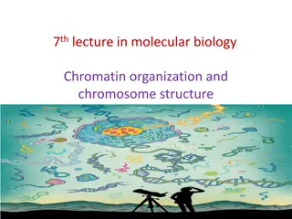
Insights into 3D Chromatin Conformation Analysis
Chromatin conformation analysis is crucial for understanding gene expression dynamics. Today's program covers topics such as 3D chromatin organization, Hi-C method, biases in Hi-C data analysis, and integrated analysis of data sources. Techniques like Chromosome Conformation Capture Technologies and their implications on gene regulation are discussed. Exploring the highest and 50 kb resolution levels of 3D chromatin conformation provides insights into topological domain interactions and epigenetic signatures. The manual annotation of TADs enriched for active marks, Polycomb, or heterochromatin reveals the spatial organization of chromatin in the nucleus.

Uploaded on Oct 03, 2024 | 0 Views
Download Presentation

Please find below an Image/Link to download the presentation.
The content on the website is provided AS IS for your information and personal use only. It may not be sold, licensed, or shared on other websites without obtaining consent from the author. Download presentation by click this link. If you encounter any issues during the download, it is possible that the publisher has removed the file from their server.
E N D
Presentation Transcript
V6 Analyzing 3D chromatin conformation Chromatin conformation has large implications on gene expression, but is usually ignored in expression analysis. Program for today: - 3D chromatin conformation - Hi-C method - Biases in Hi-C data analysis - integrated analysis of multiple data sources V6 Processing of Biological Data - WS 2018/19 1
chromatin www.wikipedia.org V6 Processing of Biological Data - WS 2018/19 2
Chromosome Conformation Capture Technologies DNA- protein cross- links e.g. with 1-3% formaldehyde, 30 min add primers biotin tags at ligation junctions second ligation Step primer for one DNA region 2002 2006 2006 2009 www.wikipedia.org V6 Processing of Biological Data - WS 2018/19 3
3D Chromatin conformation: highest level 249 Mb 242 Mb 198 Mb 186 Mb Data from human GM12878 cells (lymphoblastoid cell line). Nucleus At the highest-level of 3D organization trans-interactions are rare and individual chromosomes (chrs) occupy distinct territories (denoted by irregular shapes) within the nucleus (grey circle). Gene-rich chromosomes are preferentially found inside the nuclear core and gene- poor chromosomes are localized close to the nuclear membrane. Bonev & Cavalli, Nature Rev Genet17, 661 678 (2016) | V6 Processing of Biological Data - WS 2018/19 4
3D Chromatin conformation: 50 kb resolution Different topological domains with similar epigenetic signatures are characterized by stronger inter-domain interactions. They are organized into compartments. Here, blue and grey represent the active compartment, whereas interactions between green, orange and red topologically associating domains (TADs) form the inactive compartment. Bonev & Cavalli, Nature Rev Genet17, 661 678 (2016) | V6 Processing of Biological Data - WS 2018/19 5
3D Chromatin conformation: 10kb resolution (left) ca. 8 Mb region containing several TADs that are manually annotated with solid lines. (right) 3 different TADs, enriched for either active marks (H3K4me3 and H3K36me3; grey), Polycomb (H3K27me3; green) or heterochromatin (H3K9me3; orange) are schematically represented in the 3D space. CTCF proteins are shown as blue rectangles and loop-extrusion complexes (potentially cohesin) are depicted as green circles. Bonev & Cavalli, Nature Rev Genet17, 661 678 (2016) | V6 Processing of Biological Data - WS 2018/19 6
3D Chromatin conformation: 5kb resolution (right) Examples of different types of chromatin loops that can potentially reside within a domain (left) : example of an architectural loop as seen in high- resolution Hi-C data (regions participating in loop formation are demarcated with dotted lines), as well as CCCTC-binding factor (CTCF)-binding profile and CTCF motif orientation. Bonev & Cavalli, Nature Rev Genet17, 661 678 (2016) | V6 Processing of Biological Data - WS 2018/19 7
Data from HiC n n contact matrix, where the genome is divided into n equally sized bins. The value within each cell of the matrix indicates the number of pair-ended reads spanning between a pair of bins. Depending on sequencing depths, the commonly used sizes of these bins can range from 1 kb to 1 Mb. The bin size of Hi-C interaction matrix is also referred to as 'resolution', Owing to high sequencing cost, most available Hi-C datasets have relatively low resolution such as 25 or 40 kb, as the linear increase of resolution requires a quadratic increase in the total number of sequencing reads. Zhang et al. Nature Commun 9, 750 (2018) V6 Processing of Biological Data - WS 2018/19 8
Biases in computational analysis of Hi-C data Procedures including crosslinking, chromatin fragmentation, biotin-labelling and re-ligation can all introduce biases that complicate the interpretation of observed contact frequencies. Efficient and effective removal of multiple systematic biases is critical for the success of any subsequent analysis of C-data as well as for the proper interpretation of results. Schmitt et al. Nature Rev Mol Cell Biol (2016) 17, 743 V6 Processing of Biological Data - WS 2018/19 9
Random collisions affect chromosome capture data Detection of an interaction between two loci does not necessarily mean that they are engaged in a functional looping interaction. -> loci along a chromatin fiber will also randomly, and quite frequently, collide as the result of the inherent flexibility of chromatin. In general, the frequency of random collisions is inversely related to the genomic distance between loci (larger search space for larger radius). Thus, relatively frequent but nonfunctional interactions should always be observed for loci separated by small distances. For sites separated by larger genomic distances, this 'background' signal decreases rapidly, but remains detectable for sites separated by as much as 150 kb. Job Dekker, Nature Methods3, 17 21 (2006) V6 Processing of Biological Data - WS 2018/19 10
Persistence length of DNA The persistence length is a basic mechanical property quantifying the stiffness of a polymer. The persistence length, P, is defined as the length over which correlations in the direction of the tangent are lost. Let us define the angle between a vector that is tangent to the polymer at position 0 (zero) and a tangent vector at a distance L away from position 0, along the contour of the chain. It can be shown that the expectation value of the cosine of the angle falls off exponentially with distance, where P is the persistence length and the angled brackets denote the average over all starting positions. Bare double-helical DNA has a persistence length of about 39 nm. For comparison, a nucleosome has dimensions of 6 10 nm. www.wikipedia.org V6 Processing of Biological Data - WS 2018/19 11
Specific contacts affect neighboring loci A specific contact between two elements located on two different chromosomes in this example between centromeres will also bring neighboring fragments into closer proximity, and thus they can nonspecifically interact. Failure to determine a local peak in interaction frequencies may result in incorrectly concluding that two elements specifically interact, whereas in reality it is their neighbors that are engaged in a specific interaction. In this example, only the interaction between the two centromeres may be specific (-> highest peak) , whereas interactions with neighboring loci are likely the result of random collisions. Job Dekker, Nature Methods3, 17 21 (2006) V6 Processing of Biological Data - WS 2018/19 12
Bias 1: restriction enzyme fragment length HindIII 78%, NcoI 88% - 2 restriction enzymes Hi-C ligation products (shown schematically in a) are expected to map near restriction sites because of size selection. (b) For each Hi-C paired read, the sum of distances is computed from mapped Hi-C sequences to the nearest restriction sites. Shown is the distribution of distances. Two distinct populations of reads are observed, one distributed as expected for normally ligated and size-selected products and one including reads mapped farther away from restriction sites. Solution: discard reads with distance > 500 bp Yaffe, Tanay Nature Genet (2011) 43, 1059 V6 Processing of Biological Data - WS 2018/19 13
Bias 2 : GC content (e) Ligation product processing and sequencing may be biased by GC content. In this example, the GC-rich region produces many more reads. (f) Plotting the GC content of the 200 bp near the restriction fragment ends for trans-contacts shows intense and contrasting GC biases for the HindIII and NcoI experiments: NcoI prefers GC-rich sequences, HindIII disfavors them. Yaffe, Tanay Nature Genet (2011) 43, 1059 V6 Processing of Biological Data - WS 2018/19 14
Bias 3 : sequence mappability (g) Effect of sequence uniqueness. Different fractions of uniquely mappable short tags are observed next to restriction sites. As shown in h, this has a direct empirical linear effect on Hi-C coverage. Mappability is predicted and confirmed (h) to have a linear effect on the estimated trans-contact probabilities. Yaffe & Tanay correct for biases 2 & 3 by a maximum likelihood approach. Yaffe, Tanay Nature Genet (2011) 43, 1059 V6 Processing of Biological Data - WS 2018/19 15
Biases in computational analysis of Hi-C data In general, there exist two types of approaches to account for biases in C-data. (1) account for biases in an explicit fashion by assuming that all sources of systematic biases are known based on biases determined empirically from the observed data. (2) account for biases in an implicit way by assuming no known source (or sources) of bias, and assuming that the cumulative effect of the bias is captured in the sequencing coverage of each locus (or bin ). As Hi-C is a genome-wide assay, the implicit models assume that each locus should receive equal sequence coverage after biases are removed. Implicit models all rely on some implementation of matrix-balancing algorithms. Schmitt et al. Nature Rev Mol Cell Biol (2016) 17, 743 V6 Processing of Biological Data - WS 2018/19 16
HiCnorm tool HiCnorm corrects for these 3 biases using Poisson regression. Poisson regression assumes that the response variable Y has a Poisson distribution, and assumes that the logarithm of its expected value can be modeled by a linear combination of unknown parameters. Hu et al. Bioinformatics 28, 3131-3133 (2012) www.wikipedia.org V6 Processing of Biological Data - WS 2018/19 17
Matrix balancing A matrix is unbalanced if the L2 norm of some rows and their corresponding columns are different by orders of magnitude. Some computations such as the computation of eigenvalues are numerically unstable if the matrix is unbalanced. Given an unbalanced matrix A, the goal of matrix balancing is to find an invertible diagonal matrix D such that DAD-1is balanced or approximately balanced in the sense that every row and its corresponding column have the same norm. Schmitt et al. Nature Rev Mol Cell Biol (2016) 17, 743 V6 Processing of Biological Data - WS 2018/19 18
Matrix balancing approaches Implicit, matrix-balancing approaches have been widely used to account for biases in Hi-C data. They rely on two different assumptions. (1) the combinatorial-bias effect between two interacting loci can be simplified as the product of the two locus-specific bias effects. (2) if there is no bias effect (that is, when all bias has been accounted for), the total genome-wide contact summation for each locus will be a constant, implying that each locus has equal visibility to the Hi-C assay. Schmitt et al. Nature Rev Mol Cell Biol (2016) 17, 743 V6 Processing of Biological Data - WS 2018/19 19
Matrix balancing approaches Two matrix-balancing algorithms are: Vanilla coverage: To account for bias, the observed contact frequency between locus A and locus B is divided by the product of the total genome-wide contact frequency at locus A and the total genome-wide contact frequency at locus B. This ratio is used as the normalized contact frequency. Iterative correction and eigenvector decomposition (ICE): this process iterates through the vanilla coverage procedure (using updated total genome-wide contact frequencies!) until there is convergence of the normalized contact frequency. + reduced coverage variability from locus to locus - greatly increased computational cost. Schmitt et al. Nature Rev Mol Cell Biol (2016) 17, 743 Imakaev et al. Nature Methods 9, 999 1003 (2012) V6 Processing of Biological Data - WS 2018/19 20
Application of 4 bias removal methods: full chromosome High-resolution Hi-C data from IMR90 cells were processed uniformly until the bias-removal step, at which point either raw contact matrices were generated or normalization was conducted with one of three methods. Shown is data for whole human chromosome 7 for a raw Hi-C contact matrix (part a), an explicit model of bias removal (HiCNorm) (part b), and two methods of matrix-balancing algorithms for bias removal, vanilla coverage (VC) (part c) and iterative correction and eigenvector decomposition (ICE) (part d). Schmitt et al. Nature Rev Mol Cell Biol (2016) 17, 743 V6 Processing of Biological Data - WS 2018/19 21
Application of 4 bias removal methods: TAD domains Pairwise interactions observed at higher frequency are depicted as a darker red colour along the colour gradient, whereas light red coloration represents very few observed interactions in the Hi-C data. Different normalization methods yield slightly differences but very different numbers. It is currently unclear which method works best. Schmitt et al. Nature Rev Mol Cell Biol (2016) 17, 743 V6 Processing of Biological Data - WS 2018/19 22
Integration of multiple data sets The group of Frank Alber/USC has originally constructed a 3D model of the nuclear pore complex via data integration. They now work on 3D models of chromatin. lamina-DamID experiments identify specific chromatin domains with a high propensity to be located at the nuclear envelope (NE). Chromosome conformation capture experiments (Hi-C and variants) detect chromatin interactions at a genome-wide scale. Li et al. Genome Biology (2017) 18:145 V6 Processing of Biological Data - WS 2018/19 23
lamina-DamID experiments Schematic illustration of DNA adenine methyltransferase identification (DamID) experimental pipeline. (a) Dam only or Dam fused to a protein of interest (POI) (blue) is expressed in a suitable cell type or transgenic organism. Here: POI is lamin B1 that is part of the nuclear lamina DAM localizes to nuclear membrane (b) Genomic DNA is extracted. DNA obtained includes N6 adenine methylation sites (Me) catalyzed by Dam. (c) Genomic DNA is digested by the methylation sensitive restriction enzyme, DpnI. (d) Digested fragments are amplified by polymerase chain reaction (PCR). (e) Representative output indicating chromatin binding of a protein of interest at an individual locus. Vertical bars indicate the log2ratio of Dam fusion/Dam only. WIREs Dev Biol (2016) 5:25 37. V6 Processing of Biological Data - WS 2018/19 24
Integration of multiple data sets So far, most population convolution models of genome structures have typically relied on just one data type, such as Hi-C, even though a single experimental method cannot capture all aspects of the spatial genome organization. However, data are available from several technologies with complementary strengths and limitations. Integrating all these different data types should increase the accuracy and coverage of genome structure models. Moreover, such models would offer a way to cross-validate the consistency of data obtained from complementary technologies. Li et al. Genome Biology (2017) 18:145 V6 Processing of Biological Data - WS 2018/19 25
Integration of multiple data sets For example, lamina-DamID experiments show a chromatin region s probability to be close to the lamina at the nuclear envelope, whereas Hi-C experiments reveal the probability that two chromatin regions are in spatial proximity. Large-scale 3D fluorescence in situ hybridization (FISH) experiments show the distance between loci directly, and can be used to measure the distribution of distances across a population of cells. Li et al. Genome Biology (2017) 18:145 V6 Processing of Biological Data - WS 2018/19 26
Drosophila melanogaster The genome of D. melanogaster (sequenced in 2000, and curated at the FlyBase database) contains 139.5 million base pairs on four pairs of chromosomes: an X/Y pair, and three autosomes labeled 2, 3, and 4. It contains around 15,682 genes. The euchromatin genome was divided into 1169 physical domains based on Hi-C interaction profiles. www.wikipedia.org V6 Processing of Biological Data - WS 2018/19 27
Integration of multiple data sets Suppose A is a probability matrix derived from Hi-C data. Its elements describe how frequently a given pair of TADs are in contact with each other in an ensemble of cells. E is a probability vector derived from lamina-DamID data. Its entries describe how frequently a given TAD is in contact with the nuclear envelope (NE). The goal is to generate a population of genome structures X, whose TAD TAD and TAD NE contact frequencies are statistically consistent with both A and E. We formulate the genome structure modeling problem as a maximization of the likelihood P(A, E|X). Li et al. Genome Biology (2017) 18:145 V6 Processing of Biological Data - WS 2018/19 28
Consider population of chromatin conformations The structure population is defined as a set of M diploid genome structures X = {X1, X2, , XM}, where the m-th structure Xmis a set of 3D vectors representing the center coordinates of 2 N domain spheres. The contact probability matrix A = (aIJ)N N for N TAD domains is derived from the Hi-C data. Each element aIJis the probability that a direct contact between domains I and J exists in a structure of the population. The contact probability vector E = {eI|I= 1, 2, , N} is derived from the lamina- DamID data and defines the probability for each TAD to be localized at the NE. Li et al. Genome Biology (2017) 18:145 V6 Processing of Biological Data - WS 2018/19 29
Integration of multiple data sets The contact indicator tensor W = (wijm) 2N 2N M is a binary, third-order tensor. It contains the information missing from the Hi-C data A, namely which domain contacts belong to each of the M structures in the model population and also which homologous chromosome copies are involved. V = (vim) 2N M specifies which domain is located near the NE in each structure of the population and also distinguishes between the two homologous TAD copies Li et al. Genome Biology (2017) 18:145 V6 Processing of Biological Data - WS 2018/19 30
Integration of multiple data sets The initial structures are random configurations. Maximum likelihood optimization is achieved through an iterative process with two steps, assignment (A) and modeling (M). We increase the optimization hardness over several stages by including contacts from the Hi-C matrix A with lower probability thresholds ( ). After the population reproduces the complete Hi-C data, we include the vector E (lamina- DamID), again in stages with decreasing contact probability thresholds ( ). Li et al. Genome Biology (2017) 18:145 V6 Processing of Biological Data - WS 2018/19 31
Snapshot of a single structure picked from final population (right) euchromatin domains are colored to reflect their epigenetic class: red, active; blue, PcG; green, HP1; dark purple, null. Heterochromatin spheres are shown in grey and the nucleolus inpink (left) The full diploid chromosomes are shown in colors: blue, chr2; green, chr3; magenta, chr4; orange, chrX. The two homologs of the same chromosome are distinguished by the color tone, with one homolog copy with lighter and one with darker color. The heterochromatin spheres are larger than the euchromatin domains. The nucleolus is colored in silver. Li et al. Genome Biology (2017) 18:145 V6 Processing of Biological Data - WS 2018/19 32
Independent control experiments (FISH) The model predicts certain location preferences for pericentromeric heterochromatin of individual chromosomes. We confirmed these predictions using FISH staining of heterochromatic repeated sequences (satellites) in Drosophila cells of larval brains. Li et al. Genome Biology (2017) 18:145 V6 Processing of Biological Data - WS 2018/19 33
Summary Chromosome capture techniques enable to obtain information on contacts along one chromosome and between chromosomes. Experimental design introduces various biases that must be corrected before analysis. Data integration has great potential. Considering populations of different structures helps to resolve conflicts between data. V6 Processing of Biological Data - WS 2018/19 34


")