FPGA Accelerator Design Principles and Performance Snapshot


CS295: Modern Systems
FPGA Accelerator Design Principles
Sang-Woo Jun
Spring, 2019

FPGA Performance and Clock Speed
Typical FPGA clock speed is much slower than CPU/GPUs
o
Modern CPUs around 3 GHz
o
Modern GPUs around 1.5 GHz
o
FPGAs vary by design, typically up to 0.5 GHz
Then how are FPGAs so fast?
o
Simple answer: Extreme pipelining via systolic arrays
FPGA Performance Snapshot (2018)
Xilinx Inc., “Accelerating DNNs with Xilinx Alveo Accelerator Cards,” 2018
*Nvidia P4 and V100 numbers taken from Nvidia Technical Overview, "Deep Learning Platform, Giant Leaps in Performance
and Efficiency for AI Services, from the Data Center to the Network's Edge
Back to Flynn’s Taxonomy
SISD
Single-Instruction
Single-Data
(Single-Core Processors)
SIMD
Single-Instruction
Multi-Data
(GPUs, SIMD Extensions)
MISD
Multi-Instruction
Single-Data
(Systolic Arrays,…)
CPU/GPU
FPGA target
Example Application:
Gravitational Force
Pipelined Implementation Details
×
×
-
sq
-
sq
+
÷
G
m
1
m
2
x
2
x
1
y
2
y
1
flip-flops/registers
Little’s Law
Floating Point Arithmetic in FPGA
Floating point operations implemented using CLBs is inefficient
o
CLB: Configurable Logic Blocks – Basic unit of reconfiguration
Xilinx provides configurable floating point “cores”
o
Uses DSP blocks to implement floating point operations
o
Variable cycles of latency – variable maximum clock speed
o
Configurable operations (+-*/…) and bit width (single/double/other)
o
e.g., Single-precision (32-bits) floating point multiplication can have 7 cycles of
latency for the fastest clock speed/throughput
Floating Point Arithmetic in FPGA
a,b
×
c
Floating Point Arithmetic in Bluespec
FloatMult#(8,23) mult1 <- mkFloatMult;
FloatMult#(8,23) mult2 <- mkFloatMult;
FIFO#(Float) cQ <- mkSizedFIFO(7);
rule
step1;
Tuple3
#(Float,Float,Float) a = inputQ.first;
inputQ.deq;
cQ.enq(tpl_3(a));
mult1.put(tpl_1(a),tpl_2(a));
endrule
rule
step2;
Float r <- mult1.get;
cQ.deq;
mult2.put(r, cQ.first);
endrule
rule
step3;
let r <- mult2.get;
outputQ.enq(r);
endrule
Forwarding stages abstracted
using a FIFO
o
FIFO length doesn’t have to
exactly match latency – Only
has to be larger
o
Latency-insensitive (or less
sensitive design)
Another example:
Memory/Network Access Latency
Round-trip latency of DRAM/Network on FPGA is in the order of
microseconds
Let’s assume 2 us network round-trip latency, FPGA at 200 MHz
o
Network latency is 200 cycles
o
Little’s law means 200 requests must be in flight to maintain full bandwidth,
meaning the forwarding pipeline must have more than 200 stages
o
mkBRAMFIFO
req
Network
resp
…
Request context forwarded
time
Replicating High-Latency Pipeline Stages
Some pipeline stages may inherently have high latency, but cannot
handle many requests in flight at once
o
The GCD module from before is a good example
o
Replicate the high-latency pipeline stage to handle multiple requests at once
Example: In-memory sorting
o
Sorting 8-byte element in chunks of 8 KB (1024 elements)
o
Sorting module using binary merge sorter requires 10 passes to sort 8 KB
•
1024*9 cycle latency (last pass can be streaming)
•
Little’s law says we need 1024*9 elements in flight to maintain full bandwidth
•
Sorter module needs to be replicated 9 times to maintain wire-speed
Roofline Model
Simple performance model of a system with memory and processing
Performance is bottlenecked by either processing or memory bandwidth
o
As compute intensity (computation per memory access) increases, bottleneck
moves away from memory bandwidth to computation performance
o
Not only FPGAs, good way to estimate what kind of performance we should be
getting in a given system
We don’t want our computation
implementation to be the bottleneck!
Goal: Saturate PCIe/Network/DRAM/etc
Analysis of the Floating Point Example
Computation: a*b*c
Let’s assume clock frequency of 200 MHz
Input stream is three elements (a,b,c) per cycle = 12 Bytes/Cycle
o
200 MHz * 12 Bytes = 2.4 GB/s
o
Fully pipelined implementation can consume data at 2.4 GB/s
o
If we’re getting less than that, there is a bottleneck in computation!
What if we want more than 1 tuple/cycle?
o
Simple for this example, as computation is independent: replicate!
Performance of Accelerators
Factors affecting accelerator performance
o
Throughput of the compute pipeline
•
Can it be replicated? (Amdahl’s law? Chip resource limitations?)
o
Performance of the on-board memory
•
Is it sequential? Random? (Latency affects random access bandwidth for small memory systems
with few DIMMs) – Effects may be order of magnitude
•
Latency bound?
o
Performance of host-side link (PCIe?)
•
Latency bound?
Any factor may be the critical bottleneck
“Discrete signal processing filter whose response to a signal is of finite
length”
Simple intuition: Each output of the filter is a weighted sum of N most
recent input values
o
Convolution of a 1D matrix on a streaming input
o
Used to implement many filters including
low-pass, band-pass, high-pass, etc
o
Weights are calculated using Discrete Fourier Transforms, etc
Example:
Finite Impulse Response (FIR) Filter
Pipelining an
Finite Impulse Response (FIR) Filter
Every pipeline stage multiplies x[i]*b[j] and forwards accumulated result
If add or multiply takes multiple cycles, forwarding queue needs to be
sized appropriately
What if in/out is wide: multiple elements per cycle?
o
b[0]*x[i]+b[1]*x[i-1] is forwarded instead
b[1]
x[i]
b[2]
b[3]
in
b[0]
×
×
×
×
+
out
+
+
Pipelined tree of adders
Pipelined chain of multipliers
This content explores the principles behind FPGA accelerator design, highlighting the extreme pipelining via systolic arrays that enables FPGAs to achieve high speeds despite lower clock frequencies compared to CPUs and GPUs. It delves into the application of Flynn's Taxonomy, performance snapshots from Xilinx and Nvidia, and discusses the efficiency of floating-point arithmetic in FPGAs. Overall, the focus is on showcasing how FPGAs achieve fast processing through innovative design approaches.
- FPGA Accelerator Design
- Performance Snapshot
- Systolic Arrays
- Flynns Taxonomy
- Floating-point Arithmetic

Download Presentation

Please find below an Image/Link to download the presentation.
The content on the website is provided AS IS for your information and personal use only. It may not be sold, licensed, or shared on other websites without obtaining consent from the author. Download presentation by click this link. If you encounter any issues during the download, it is possible that the publisher has removed the file from their server.
E N D
Presentation Transcript
CS295: Modern Systems FPGA Accelerator Design Principles Sang-Woo Jun Spring, 2019
FPGA Performance and Clock Speed Typical FPGA clock speed is much slower than CPU/GPUs o Modern CPUs around 3 GHz o Modern GPUs around 1.5 GHz o FPGAs vary by design, typically up to 0.5 GHz Then how are FPGAs so fast? o Simple answer: Extreme pipelining via systolic arrays
FPGA Performance Snapshot (2018) Xilinx Inc., Accelerating DNNs with Xilinx Alveo Accelerator Cards, 2018 *Nvidia P4 and V100 numbers taken from Nvidia Technical Overview, "Deep Learning Platform, Giant Leaps in Performance and Efficiency for AI Services, from the Data Center to the Network's Edge
Back to Flynns Taxonomy SISD Single-Instruction Single-Data (Single-Core Processors) SIMD Single-Instruction Multi-Data (GPUs, SIMD Extensions) MISD Multi-Instruction Single-Data (Systolic Arrays, ) CPU/GPU FPGA target
Example Application: Gravitational Force ? ?1 ?2 (?1 ?2)2+(?1 ?2)2 8 instructions on a CPU 8 cycles* o One answer per 8 cycles o Ignoring load/store FPGA: Pipelined systolic array o One answer per 1 cycle o 200 MHz vs. 3 GHz makes a bit more sense! o Very simple systolic array We can fit a lot into a chip Unlike cache-coherent cores - sq - sq + t=0 t=1 t=2 t=3 t=4 t=5 t=6 t=7
Pipelined Implementation Details ? ?1 ?2 (?1 ?2)2+(?1 ?2)2 G m1 m2 x1 - sq - sq + x2 y1 y2 flip-flops/registers
Littles Law ? = ?? o L: Number of requests in the system o ?: Throughput o W: Latency Simple analysis: Given a system with latency W, in order to achieve throughput, we need to be processing as many things as possible
Floating Point Arithmetic in FPGA Floating point operations implemented using CLBs is inefficient o CLB: Configurable Logic Blocks Basic unit of reconfiguration Xilinx provides configurable floating point cores o Uses DSP blocks to implement floating point operations o Variable cycles of latency variable maximum clock speed o Configurable operations (+-*/ ) and bit width (single/double/other) o e.g., Single-precision (32-bits) floating point multiplication can have 7 cycles of latency for the fastest clock speed/throughput
Floating Point Arithmetic in FPGA Simple example: a b c o Uses two multiplier cores, 7 cycle latencies each o c also needs to be forwarded via 7 pipelined stages What happens if c has less than 7 forwarding stages? o From ? = ??: If we have L = 4, W = still 7 ?=4/7 c a,b
Floating Point Arithmetic in Bluespec FloatMult#(8,23) mult1 <- mkFloatMult; FloatMult#(8,23) mult2 <- mkFloatMult; FIFO#(Float) cQ <- mkSizedFIFO(7); rule step1; Tuple3#(Float,Float,Float) a = inputQ.first; inputQ.deq; cQ.enq(tpl_3(a)); mult1.put(tpl_1(a),tpl_2(a)); endrule rule step2; Float r <- mult1.get; cQ.deq; mult2.put(r, cQ.first); endrule rule step3; let r <- mult2.get; outputQ.enq(r); endrule Forwarding stages abstracted using a FIFO o FIFO length doesn t have to exactly match latency Only has to be larger o Latency-insensitive (or less sensitive design)
Another example: Memory/Network Access Latency Round-trip latency of DRAM/Network on FPGA is in the order of microseconds Let s assume 2 us network round-trip latency, FPGA at 200 MHz o Network latency is 200 cycles o Little s law means 200 requests must be in flight to maintain full bandwidth, meaning the forwarding pipeline must have more than 200 stages o mkBRAMFIFO time Network req resp Request context forwarded
Replicating High-Latency Pipeline Stages Some pipeline stages may inherently have high latency, but cannot handle many requests in flight at once o The GCD module from before is a good example o Replicate the high-latency pipeline stage to handle multiple requests at once Example: In-memory sorting o Sorting 8-byte element in chunks of 8 KB (1024 elements) o Sorting module using binary merge sorter requires 10 passes to sort 8 KB 1024*9 cycle latency (last pass can be streaming) Little s law says we need 1024*9 elements in flight to maintain full bandwidth Sorter module needs to be replicated 9 times to maintain wire-speed
Roofline Model Simple performance model of a system with memory and processing Performance is bottlenecked by either processing or memory bandwidth o As compute intensity (computation per memory access) increases, bottleneck moves away from memory bandwidth to computation performance o Not only FPGAs, good way to estimate what kind of performance we should be getting in a given system We don t want our computation implementation to be the bottleneck! Goal: Saturate PCIe/Network/DRAM/etc
Analysis of the Floating Point Example Computation: a*b*c Let s assume clock frequency of 200 MHz Input stream is three elements (a,b,c) per cycle = 12 Bytes/Cycle o 200 MHz * 12 Bytes = 2.4 GB/s o Fully pipelined implementation can consume data at 2.4 GB/s o If we re getting less than that, there is a bottleneck in computation! What if we want more than 1 tuple/cycle? o Simple for this example, as computation is independent: replicate!
Performance of Accelerators Factors affecting accelerator performance o Throughput of the compute pipeline Can it be replicated? (Amdahl s law? Chip resource limitations?) o Performance of the on-board memory Is it sequential? Random? (Latency affects random access bandwidth for small memory systems with few DIMMs) Effects may be order of magnitude Latency bound? o Performance of host-side link (PCIe?) Latency bound? Any factor may be the critical bottleneck
Example: Finite Impulse Response (FIR) Filter Discrete signal processing filter whose response to a signal is of finite length Simple intuition: Each output of the filter is a weighted sum of N most recent input values o Convolution of a 1D matrix on a streaming input o Used to implement many filters including low-pass, band-pass, high-pass, etc o Weights are calculated using Discrete Fourier Transforms, etc
Pipelining an Finite Impulse Response (FIR) Filter Every pipeline stage multiplies x[i]*b[j] and forwards accumulated result If add or multiply takes multiple cycles, forwarding queue needs to be sized appropriately What if in/out is wide: multiple elements per cycle? o b[0]*x[i]+b[1]*x[i-1] is forwarded instead Pipelined tree of adders + out + + b[0] b[1] b[2] b[3] in Pipelined chain of multipliers x[i]


")