Understanding Atmospheric Physics: Ideal Gas Law and Maxwellian Distribution

Exploring the physics of gases in planetary atmospheres, this lecture delves into the ideal gas law which relates pressure, density, and temperature in an atmosphere. It introduces the concept of kinetic temperature and Maxwellian distribution, showcasing how gas particles distribute in equilibrium. By analyzing characteristic speeds and their connection to planetary atmospheres, we gain insights into gas particle velocities and their relation to escaping the atmosphere.

Download Presentation

Please find below an Image/Link to download the presentation.
The content on the website is provided AS IS for your information and personal use only. It may not be sold, licensed, or shared on other websites without obtaining consent from the author. Download presentation by click this link. If you encounter any issues during the download, it is possible that the publisher has removed the file from their server.
E N D
Presentation Transcript
Physics 320: Physical Processes: Atmospheres (Lecture 13) Dale Gary NJIT Physics Department
Atmospheres We will learn later about atmospheric structure in some detail for each of the planets. Here we just want to look at some useful relationships for atmospheres, which basically means looking at the physics of gases. We start with the ideal gas law, which gives the relationship between pressure, density, and temperature for an atmosphere: ? = ??? Here P is the pressure (force per unit area, or N/m2), n is the gas number density (particles per m3), k = 1.38 x 10⁻²³J / K is Boltzmann's constant, and T is the gas temperature in K. c.f. ?? = ?mol?? The ideal gas law is based on the idea of kinetic temperature, which describes a distribution of speeds of the gas molecules (or atoms) in terms of temperature. A hot gas has faster moving particles than a cold gas. The thermal distribution is an equilibrium distribution (called the Maxwellian distribution). Video showing Maxwellian Distribution October 23, 2018
Characteristic Speeds of Maxwellian Imagine firing a beam of particles, all with the same energy, into a trap and allowing them to come into equilibrium by colliding elastically. Due to standard probability and statistics (akin to coin-tossing), they will wind up with a gaussian distribution of speeds (a bell curve). Any distribution of particles in equilibrium will have such a curve, which can be parametrized by a single number, the temperature. Due to the 3D nature of velocity, the gaussian when expressed in terms of speed becomes: 1 2??2??4??2 3/2? ???? = ? ? 2??? ?? The important dependence is the argument of the exponential, which is just the ratio of the kinetic energy (1 between ? and ? + ??. Important relationships: Peak of distribution (most probable speed) is when 1 ??= 2??/?1/2 ??= 2 1.38 10 23 300/(32 1.67 10 27) = 394 m/s 2??2) to thermal energy (kT ). This expression is the number of particles per unit volume having speeds Mass of O2 molecule 2??2= ??, or Root mean square speed is somewhat higher (due to asymmetry in the curve) ?rms= 3??/?1/2 ?rms= 3 1.38 10 23 300/(32 1.67 10 27) = 482 m/s ? = ? ? = 1 ? = 2 ? October 23, 2018
Connection to Atmospheres The way that we can connect this to planetary atmospheres is to think about the speeds of the gas particles making up the atmosphere, relative to the escape speed that we introduced before (the speed needed to escape the gravity well of a planet) 1/2 2?? ? ?esc= Recall that this just comes from equating the kinetic energy of a projectile to its potential energy at the surface of the planet: 1 2??2= ???/? If a gas has a temperature such that ?rms= ?esc, then the gas will leave the atmosphere in only a few days. To retain an atmosphere for several billion years (the age of the solar system is about 4.5 billion years), a planet must have ?esc> 6?rms heavy The factor of 6 takes into account the high-speed tail of the Maxwellian Distribution. lighter lightest The high-speed tail is sort of a leak in the atmosphere October 23, 2018
Composition of Planetary Atmospheres Planetary atmospheres contain different gases partly depending on what gases they can retain over their lifetimes. The diagram at right shows the speed 6?rms for various atoms and molecules vs. temperature, shown as diagonal dashed lines. The typical temperatures of the atmospheres and the escape speeds of planets are shown as dots. For example, the Earth s temperature is about 300 K, and the escape speed is about 11 km/s. So we would predict that the Earth can retain water, ammonia, and methane, but not helium or hydrogen. The Moon has about the same temperature as Earth, but its escape speed is much lower, so it cannot retain molecules like carbon dioxide, oxygen, or water. October 23, 2018
Composition of Planetary Atmospheres Let s check the calculation for O2 on the Moon: 2(6.67 10 11)(7 1022) 1.78 106 2?? ? ?esc= = = 2.32 km/s 3(1.38 10 23)(300) (32)(1.67 10 27) 3?? ? ?rms= = = 0.482 km/s So the escape speed is only 4.8 times the rms speed. This is less than the required 6 ?rms. We conclude that the Moon will lose any oxygen that might be produced, after only a few hundred years. Any atoms lingering around the Moon, produced due to outgassing or spalation from rocks, lasts only for a short time and must be continually replenished. The atmosphere of the Moon is an amazingly good vacuum, only 10 14 atm. The Earth's atmosphere would have started out to be mostly H and He, but lost it due to the speed of these particles allowing them to escape over time. A new, heavier atmosphere of H2O, O2, N2, and CO2 was outgassed from volcanism, or brought here by comets. October 23, 2018
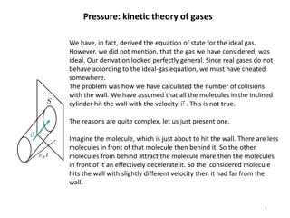
Hydrostatic Equilibrium We will now derive some important relations for atmospheres, starting with the equation of hydrostatic equilibrium. Pressure is force/unit area, F / A. Pressure in the atmosphere of a planet arises from the inward force of gravity--balanced by the outward pressure due to the normal force of the gas below it. Atmospheres can be considered as static, meaning that they are not expanding or contracting. Such a state is called hydrostatic equilibrium, and like all equilibrium situations, it is characterized by force balance. Consider a column of cross-sectional area A. The forces on a section (parcel) of the column are shown in the figure on the left. The mass of the parcel is related to the mass density by ? = ?/? = ?/?(?2 ?1). From the free-body diagram it is clear that ?1 = ?2 + ?? = ?2 + ?(?2 ?1)?? Here g is the local acceleration of gravity (which in general varies with depth in the atmosphere, but for a thin atmosphere it can be taken as constant). This force equation can be rearranged to ? / ? = ? = ??? Here ? is the pressure difference (?1 ?2) on the two ends of the column section, and ? is the radius difference, or thickness of the parcel, (?1 ?2). Taking lim ? 0 ? ? ?? ??= ?? October 23, 2018
Pressure Scale Height Now we combine that relation with the Ideal Gas Law: Here n is the number density (number of particles per unit volume), related to the mass density by ? = ?/? (? is the mass/particle). Thus, we can write ? in terms of ?, and get a new equation for ?: ?? ??= ? ?? ?? ? = ??? ?? ?? ?= ?? ?? This equation has the solution: ? = ?0? ?? ??? Here ? = (? ?0) is the height above the surface of the Earth. Thus, we can identify a pressure scale height, ? = ??/?? = constant The scale height ? is the distance over which the pressure falls from its initial pressure by a factor of 1/?. The scale height for the Earth's surface is roughly 8 km, although note that to get this result we had to assume that the temperature ? does not change with height. This is not true for Earth's atmosphere -- ? falls with height (near the surface), so that the scale height is lower. Still, the concept of a scale height is useful for atmospheres, oceans, and even the interior of solid bodies. Next semester we will again use it to describe the atmospheres of stars. October 23, 2018
Earths Atmospheric Structure At right is a plot of the temperature vs. height of the Earth s atmosphere (which we had to assume was constant in the previous discussion). Why does the temperature of the atmosphere drop to a height of about 10 km, then start to rise again in the Stratosphere? This is due to absorption of ultraviolet (UV) light from the Sun, which deposits energy in this region of the atmosphere, and heats it. This region is called the Stratosphere, because it is stable to upward motions (an inversion layer), which means that clouds do not rise in columns, but spread out in thin layers, like strata. Up to the Mesopause, the temperature again declines, but then rises again in the Thermosphere this time due to absorption of X-rays from the Sun. This "atmosphere" is only slightly below the height of low Earth orbiting satellites such as the Space Shuttle, which orbits about 200 km up. October 23, 2018
Earths Magnetosphere A planet can also have a magnetosphere, if it has appreciable magnetic fields. The rotating liquid metallic core of the Earth generates a magnetic field that, at the surface, primarily looks like a dipole (a North-South magnetic pole), although there are higher-order multipole (quadrupole, etc.) components as well. A dipole field falls off in strength as ? = ?0(?/? ) 3 The North geographic pole of the Earth actually is a South magnetic pole. This means that the direction of the fieldlines is out of the Earth at the South geographic pole, and into the Earth at the North geographic pole. At the surface of the Earth, the magnetic field strength is about 0.4 gauss, or ?0= 4 10 5 T (tesla is the SI unit). The magnetic fields reach far out into space, and surround the Earth in a Magnetosphere Radiation Belts Particle Motions Look at a real time monitoring of the magnetosphere protective region called the magnetosphere. Look at a real time monitoring of the magnetosphere. Look at a real time monitoring of the magnetosphere October 23, 2018
Gyroradius and Particle Motions One can calculate the size of the circle executed by a charged particle of a given speed, from: ? = ??/?? Example: For a proton with speed ? = 107 m/s, in field of ? = 10 5 ? the gyroradius is: ? = ??/?? = (1.67 10 27 kg)(107 m/s) / (1.60 10 19?)(10 5?) = 10.4 km This means that such a proton will execute a circular gyration path of radius 10 km. If it travels inward along the magnetic field toward one of the poles, the magnetic field strength goes up, and it spirals in a smaller circle. It will be mirrored if the field strength gets high enough, and it ends up trapped, bouncing forever from pole to pole, and drifting around the Earth. October 23, 2018
What Weve Learned You should have a good intuitive sense of the statistical properties of a Maxwellian distribution that it is characterized by a single number, the temperature, but represents a velocity distribution of particles. In particular, you should know the most probably speed (at the peak), and the mean (rms) speed, and how they depsnd on particle mass and temperature: You should understand that planets can only hold on to species gravitationally if their mean (rms) speed is at least 6 times lower than the escape speed: You should be able to use these relationships to determine what atoms or molecules a given body can be expected to have in its atmosphere. You should be able to apply the concept of pressure scale height to determine how fast the atmosphere should fall off with height: ? = ?0? ?? ??= 2??/?1/2 ?rms= 3??/?1/2 ?esc> 6?rms ? = ??/?? ??? You should know the temperature structure of the Earth s atmosphere, and the reasons for the stratosphere and mesosphere, temperature inversions due to heat input from UV and X-rays, respectively. You should understand the basics of the magnetosphere, and how to calculate the dipole magnetic field strength at any height given B0: ? = ?0(?/? ) 3 October 23, 2018