Advanced Techniques in Multivariate Approximation for Improved Function Approximation

Explore characteristics and properties of good approximation operators, such as quasi-interpolation and Moving Least-Squares (MLS), for approximating functions with singularities and near boundaries. Learn about direct approximation of local functionals and high-order approximation methods for non-smooth multivariate functions. Discover how these advanced techniques enhance approximation accuracy and efficiency in various applications.

• Multivariate Approximation
• Function Approximation
• Moving Least-Squares
• High-Order Approximation
• Singularities

bade_ife Follow

Uploaded on Oct 09, 2024 | 0 Views

Download Presentation

Please find below an Image/Link to download the presentation.

The content on the website is provided AS IS for your information and personal use only. It may not be sold, licensed, or shared on other websites without obtaining consent from the author. Download presentation by click this link. If you encounter any issues during the download, it is possible that the publisher has removed the file from their server.

Presentation Transcript

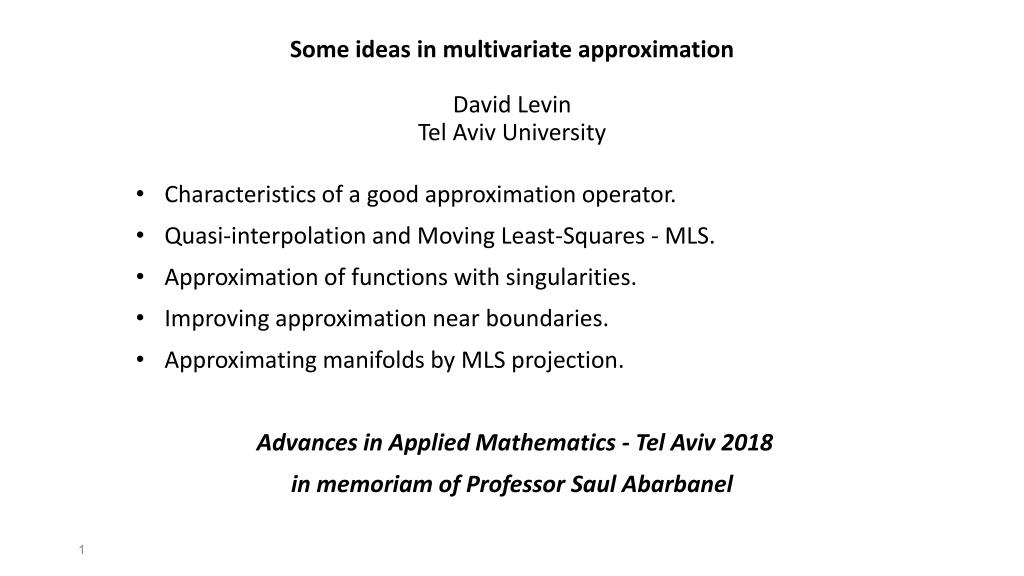
1. Some ideas in multivariate approximation David Levin Tel Aviv University Characteristics of a good approximation operator. Quasi-interpolation and Moving Least-Squares - MLS. Approximation of functions with singularities. Improving approximation near boundaries. Approximating manifolds by MLS projection. Advances in Applied Mathematics - Tel Aviv 2018 in memoriam of Professor Saul Abarbanel 1

2. Characteristics of a good approximation operator Given function values at scattered points {??} in ? ??, we want to approximate the function at any point x in ?. Linear approximations operators are of the form: ? Qf(x)= ?=1 ??(x)f(??) . Desired properties of the coefficients {??(x)} : A. Reconstruction of a specific subspace (e.g., polynomials). B. Locality (finite support ). C. Smoothness. ? , A+B imply: The approximation error at x is bounded by ?=1 is the error of the best sup-norm approximation to f over . |??? |? ? 2

3. ? Qf(?) )= ?=? ??( (x) x)f( f(??) ) Desired properties of Qf( A. Reconstruction of a specific subspace (e.g., polynomials), ? Qp(?)= ?=1 ??(?)p(??) = ? ? , ? ??, ? ? . ? 2(?)? B. Locality , minimize ?=1 where ?(r) is fast increasing with r ( e.g. : ?(r) = ???2). ?? ? ?? C. Smoothness, Solving A+B for {??(x)} , smoothness follows if ?(r) is smooth. The result is the Moving Least-Squares approximation MLS with the weight function w r = 1/?(r) . Such approximations are called Quasi-interpolation approximations. 3

4. Direct approximation of local functionals In many applications we want to approximate derivatives or integrals over elements. Instead of differentiating or integrating the MLS approximation, we can obtain it directly as follows : To approximate a functional ?[?](?), we look for an approximation of the form ? Tf(x)= ?=1 ??(x)f(??) with the properties A. Reconstruction of the functional over a specific subspace , ? Tp(?)= ?=1 ??(?)p(??) = ?[?] ? , ? ??, ? ? . B. Locality , ? 2(?)? minimize ?=1 ?? ? ?? where ?(r) is fast increasing with r. 4

5. High order approximation to non-smooth multivariate functions joint work with Anat Amir, CAGD 2018 Quasi-interpolation to non-smooth functions achieves low approximation orders near the singularities of the function or its derivatives. The idea is to use the structure of the high errors near singularities. We identify the type and the location of the singularity, and correct the quasi-interpolation to retrieve full approximation order. Original errors: Errors after correction: 5

6. High order approximation near boundaries joint work with Anat Amir Most approximation methods exhibits large errors near the boundaries of the data domain. Here again, the structure of the errors of the quasi-interpolation approximation near the boundaries can be used to improve the approximation near the boundaries. 6

7. Approximating manifolds from noisy data no order, no parametrization. An MLS projection approach: 1. Approximate a local coordinate system. 2. Use MLS approximation w.r.t. the local coordinate system. An example - Noisy data of a curve in 3D: 7

8. Same example - Noisy data of a curve in 3D. Applying the projection operator to all data points: Joint work with Barak Sober 8

9. Same example - Noisy data of a curve in 3D Thank you! 9