Understanding Machine Learning: Types and Approaches
Machine learning involves various types of learning strategies, ranging from skill refinement to knowledge acquisition. This spectrum includes caching, chunking, refinement, and knowledge acquisition. Differentiating between supervised and unsupervised learning, understanding how machines learn is pivotal in AI development.

Download Presentation

Please find below an Image/Link to download the presentation.
The content on the website is provided AS IS for your information and personal use only. It may not be sold, licensed, or shared on other websites without obtaining consent from the author. Download presentation by click this link. If you encounter any issues during the download, it is possible that the publisher has removed the file from their server.
E N D
Presentation Transcript
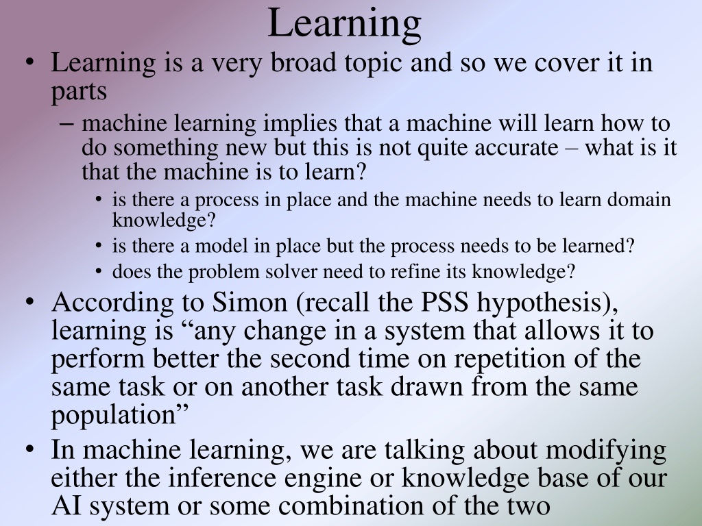
Learning Learning is a very broad topic and so we cover it in parts machine learning implies that a machine will learn how to do something new but this is not quite accurate what is it that the machine is to learn? is there a process in place and the machine needs to learn domain knowledge? is there a model in place but the process needs to be learned? does the problem solver need to refine its knowledge? According to Simon (recall the PSS hypothesis), learning is any change in a system that allows it to perform better the second time on repetition of the same task or on another task drawn from the same population In machine learning, we are talking about modifying either the inference engine or knowledge base of our AI system or some combination of the two
A Spectrum of Types Learning encompasses a vast spectrum of types At one extreme is skill refinement the system already knows how to solve a given problem but through experience it improves either by becoming more efficient at the task or more accurate (or even across a wider range of problems) At the other extreme is knowledge acquisition the system does not have the proper knowledge in place and must learn it this might be learning from scratch, or adding related knowledge to what it already knows for instance, a medical diagnostic system may know about liver disease but then expands to learn about heart disease
Spectrum of Learning Types Caching and new cases: just adding input- output combinations Chunking possibly generalizing of what a group of I/O cases convey Refinement adjustment what we already know to improve usually done while problem solving based on feedback Knowledge acquisition learning beyond what we already know may be done while problem solving, more often done based on reading or when introduced to a new topic
Another Way to View Learning Supervised when learning, is someone giving you feedback? You did this wrong Or more specifically, this is where you went wrong And possibly accompanies by feedback that tells you how to solve the problem Unsupervised no feedback You are given enough information/knowledge to discover your own internal structures of the information/knowledge Humans learn using both approaches but humans start with a base of knowledge to build upon In AI, supervised learning is far easier than unsupervised learning and unsupervised learning may not actually accomplish what we want
What We Will Study There are many different algorithms and approaches for learning based on what type of knowledge representation is being used In this chapter, we focus on symbolic learning learning concepts that are represented symbolically we start by looking at two inductive forms representations are learned by examining positive and negative instances one at a time In chapter 11, we focus on subsymbolic forms of learning (neural networks) In chapter 12, we focus on the genetic algorithm and its related forms this may or may not be considered learning In chapter 13, we look at probabilistic forms of learning, which may or may not be considered learning as well
Learning Within a Concept Space Consider: we already know a concept space the features used to represent classes (and the range of values each feature can take on) our task is to learn the proper values for the features for a given class/concept by examining a series of examples This is inductive learning Winston introduced an approach in the 1970s using semantic network representations instances are hits and near misses of a class working one example at a time, a class representation is formed by manipulating a target semantic network generalizing the network when a positive instance is examined specializing the network when a negative instance is examined he used the blocks world domain, and his famous example is to represent what makes up an arch using three blocks
Learning the Arch Concept We start with a description of an arch in part a and introduce a second arch in part b, using knowledge that both a brick and a pyramid are polygons, we generalize to part d A near miss is shown above in part b allowing us to specialize in part c
Version Space Search Mitchell offered an improved learning approach called Candidate Elimination similar to Winston s but with two representations a general description (G) of the concept specialized to avoid containing any negative examples a specific description (S) of the concept generalized to encompass all positive examples process iterates over + and - examples specialize G with - ex generalize S with + ex until the two representations are equal or until they become empty, in which case the examples do not lead to a single representation for the given class
How It Works There are generalization operators replace a constant with a variable color(ball, red) color(X, red) drop a condition shape(X, round) ^ size(X, small) ^ color(X, red) shape(X, round) ^ color(X, red) add a disjunct shape(X, round) ^ size(X, small) ^ color(X, red) shape(X, round) ^ size(X, small) ^ (color(X, red) v color(X, blue)) replace a property with a more generalized version color(X, red) color(X, primary_color) in the arch example, we used this to go from an instance that was a brick and an instance that was a pyramid to the more generic polygon, we need to have a predefined hierarchy of classes
Example Our domain will be of objects that have attributes of size, color shape The possible values of these attributes make up our concept space We want to learn the proper portion of the concept space that contains our positive examples and does not include any negative examples Examples to introduce might include: + small, red, ball - small, blue, ball + large, red, ball - large, red, cube
Example Continued How useful is this algorithm? After introducing positive and negative examples, we are able to represent the concept as objects that are red balls
Problems Both of the algorithms rely on having classes that can be clearly segmented by features in the concept space consider a class called good car deal which uses features of year , price , blue book value , mileage , wear and tear would we be able to form a single representation that denoted for each feature, what value(s) a good car deal should have? consider for diagnosing the flu would all patients have the same symptoms? would the patients have enough overlapping symptoms to clearly identify flu over cold or sinus infection? These two algorithms also suffer from inductive bias the order that examples are offered could influence the amount of time it takes to reach a final representation And of course, since both are search oriented processes, they suffer from combinatoric problems
LEX: Learning Heuristics To focus on a concrete example, the author shows us LEX LEX solves integration (calculus) problems through best- first search There are four operators to select between where the operators are generic and so must be unified to aspects of the current problem state e.g., convert the value 3 x2 into r x2 or 3 f(x) by unifying 3 to r or x2 to f(x) thus, there are more than 4 choices to make LEX learns and improves on heuristics to guide the best-first search LEX uses candidate elimination to take multiple heuristics that seem to be of the same family and attempts to generalize them while also removing elements of a generalized heuristic which fails to improve on the search process
How LEX Works The four operators that LEX employs are To move any constant in front of the integration To employ integration by parts To perform mathematical calculations to simplify a term To separate a sum in an integration to a sum of two (or more integrations) There are four parts to LEX generalizer to use candidate elimination on heuristics problem solver to actually perform the best-first search and apply the operators to the integration problem critic produces positive and negative heuristic instances from the problem solver for use by the generalizer problem generator to generate a new problem to solve
LEXs Hierarchy of Concepts (partial) From here, we can generalize that some constant value becomes k and some cosine function becomes trig or transandental
Concept Space For Integration by Parts LEX was able to learn heuristics that reduced its search from 200 steps to 20
Learning Decision Trees The decision tree is a tree that has questions as its nodes and conclusions as leaf nodes (diagnostic conclusions, decisions) the process is to follow a path based on user responses Quinlan introduced an inductive learning algorithm to automate the construction of decision trees given data of specific decision cases see the data to the right which shows the proper decision of whether a person is a high, moderate or low credit risk based on credit history, debt, collateral and income
The ID3 Algorithm The key to the algorithm is the selection of P, a property (feature) to subdivide the tree Selecting the wrong P will cause the algorithm to spend more time building the tree and will create a larger tree which will be less efficient
Simplified Tree In the first tree, the topmost node asked whether credit history was good, bad or unknown, but if you already know the person s income is <= 15K, it means high risk no matter what else, so using income as the first decision simplifies the tree
Information Theory Information Theory is a mathematical basis for measuring the amount of information content of a message (or data) applied in telecommunications and computer science, for instance to select a communications channel given the available carrying capacity, and applied to data compression Quinlan uses it to compute the information gain obtained by selecting a feature out of a collection of data the math gets ugly, so we will skip these details, but feel free to read about it on pages 413-415 and how we can use it to select the best feature in our credit risk data set the idea is that for each iteration in ID3 to select P, we compute the information gain of each P and select the P that has the maximum information gain, and then remove P from the data set so that it is not selected again until we get to a point in the problem solving where there are too few features left to make the computation worthwhile
ID3 Problems There are still significant problems with ID3 what if some of the data is bad, how will that impact the accuracy of the decision tree? what if features have continuous data rather than discrete values? this is a problem that is faced in data mining all the time one technique is to discretize the data by finding reasonable regions for instance by dividing income into 0-15K, 15K-35K, 35K+, identifying these regions can be computationally complex what if data is missing from the set (some of the records have no values for given features)? can we extrapolate? should we discard those records? what if the data set is too large for ID3 to handle? Quinlan has offered newer algorithms including C4.5 that get around many of these problems introducing new algorithm components: bagging and boosting (see page 417 for brief details)
Rule Induction A similar idea to decision trees is to use data to learn rules, called rule induction given a collection of data in a database analyze combinations of features to see if a generalized rule can be formed for instance, consider a database of students which includes major, minor, GPA and number of years it took to graduate when examining the data, we find the correlation that students with a CSC major and CIT minor and a GPA > 3.0 graduate in 4 or 4 years this allows us to generate a rule that we might use to predict future students performance we might even assign a probability or certainty on this rule based on the number of times it was found to be true in the database
More on Rule Induction A simple (but not efficient) algorithm for RI is For each attribute A: For each value V of that attribute: create a rule: 1. count how often each class appears 2. find the most frequent class, c 3. make a rule "if A=V then C=c" 4. calculate the error rate of this rule Pick the attribute whose rules produce the lowest error rate As an example, a store manager might use this to predict shopping behavior if a rule is generated that says if shopper buys milk and bread then the shopper will likely buy peanut butter then the manager may decide to place the peanut butter in the same aisle as the bread or the manager might run a special whereby if you buy milk and bread, your peanut butter is discounted
Learning New Concepts Our algorithms so far have learned concepts within an already established concept space What about learning some new concept that is outside of what we already know? Two approaches are presented in the text learning of new rules to explain problem solutions (Meta- DENDRAL) and explanation-based learning both approaches require some predefined concept space but not merely learning classes through identifying features This follows more closely with scientific learning you already understand some concepts, now you build upon the domain by learning new concepts consider that you first learned about loops and then you learned about infinite loops by building on your loop knowledge we are instead adding new pieces of knowledge to the model/concept space itself
Meta-Dendral Dendral was the first expert system, built in the mid 1960s it worked with a chemist to identify the chemical composition of some molecules based on the output of a mass spectrometer Dendral uses constraint satisfaction search along with a series of chemistry rules, and the chemist also input constraints to reduce the search Dendral rules are based on identifying sites of cleavage in the molecule using a theory that is incomplete (so that it cannot account for the entire identification task) Meta-Dendral takes the output of a Dendral session of some known substance, and attempts to established new cleavage rules to add to Dendral some example rules in Dendral are: double and triple bonds to not break only fragments larger than two carbon atoms show up in the data Dendral will add rules to specialize a pattern such as adding an atom to a rule such as x1*x2 (two atoms with a cleavage between them) to X3 X1*X2 (where means a chemical bond) instantiating an atom to a specific element such as X1*X2 C*X2
Explanation-Based Theory Consider as a computer science student that you first learn about control structures (loops, selection statements) and then learn specifically about while loops and then you learn about infinite loops You start with a model of the material to be learned, and then you learn a new concept (infinite loops) you are shown an example or two along with an explanation and now you have a new concept in your model EBL requires a target concept what the learner is attempting to form a new representation for a training example a domain theory (a model) operationality criteria a representation for the example and model so that the new example can be understood within the context of what has already been learned
Example: Learning what a Cup is Given the following domain theory liftable(X) & holds_liquid(X) cup(X) part(Z, W) & concave(W) & points_up(W) holds_liquid(Z) light(Y) & part(Y, handle) liftable(Y) small(A) light(A) made_of(A, features) light(A) We are given a training example: cup(obj1), small(obj1), part(obj1, handle), owns(bob, obj1), part(obj1, bottom), part(obj1, bowl), points_up(bowl), concave(bowl), color(obj1, red) Automated theorem proving can construct an explanation of why obj1 is an example of the training concept first, derive a proof that the example is a cup next, remove any irrelevant portions of the proof (e.g., owner, color) finally, the remaining axioms consist of an explanation of how the example fits the domain theory definition of a cup see the next two slides
How do we use EBL? Consider building an automated programming system (an expert system that can write new programs) We have already implemented a representation for control structures when to use them, how they work, the control mechanisms (number of iterations, loop indices, terminating conditions) Now we want to teach the system what an infinite loop is so that it won t ever write one the domain theory for loops includes loop variable(s) loop variable(s) initialization loop variable(s) increment loop termination condition that tests the loop variable(s) the concept to introduce is that the loop variable incrementing moves the loop variable(s) closer to the loop termination condition As an example of an infinite loop we offer loop_variable(x), loop_variable_initialization(x=0), loop_variable_increment(x++), loop_termination_condition(x<0)
Analogical Reasoning EBL is based on deduction anything newly learned could actually have been discovered by exhaustive search of the axioms presented We want to be able to learn beyond what we already knew one approach is through analogical reasoning reasoning by analogy unlike EBL, what we learn through analogical reasoning is not necessarily correct (it is not logically sound) the idea is that we have some source set of knowledge such as a previous problem solution, a theory that is partially understood (represented), a target concept in mind, and a set of transforms We apply a transform to the previous case to derive a new piece of knowledge whether the new piece of knowledge is useful, relevant or even true may not be knowable in general, nor may a system be able to infer whether the new piece of knowledge is useful
This is Like CBR The process is one of retrieving a previous solution from a library of solutions elaborating upon the solution to derive features of use for the target mapping (transforming) the previous solution into the target domain justifying (determining) if the mapping was valid and useful indexing and storing the newly learned piece of knowledge But CBR s result can be tested to see if it solves the given problem, here we are using the same approach to generate a new piece of knowledge is the knowledge relevant and useful? how do we perform the justification step? we also have to be careful, since we are taking knowledge from a different domain, that we don t try to be too literal with the analogy
Example Consider that we already know about the solar system with such concepts as Sun and earth, attraction (gravity), orbit, mass and heat we want to learn that an atom is like the solar system that is, both systems have similar properties we have the following source knowledge: yellow(sun), blue(earth), hotter_than(sun, earth), causes(more_massive(sun, earth) attract(sun, earth), causes(attract(sun, earth), revolves_around(earth, sun)) the target domain includes: more_massive(nucleus, electron) and revolves_around(electron, nucleus) For us to learn something useful, we can t merely map from the source to target because we will obtain incorrect or irrelevant information (such as a nucleus is yellow) mapping rules must constrain what is generated properties are dropped from the source relations are mapped unchanged but higher-order relations are preferred to lower-order relations so that relations may be dropped
Analogical Mapping So we start with two pieces of knowledge in our target more_massive(nucleus, electron) and attract(nucleus_electron) And we use a previously known piece of domain knowledge about the solar system and learn the following
Example System To understand how we can automate this, we consider the VivoMind Analogy Engine (VAE) conceptual graphs are used for knowledge representations previous human analogies are represented to find an analogy, VAE uses three methods of comparison (separately or in combination) matching type labels to see if two items have a class/subclass relationship of some kind matching subgraphs where a match is successful if two subgraphs are isomorphic (the two graphs match aside from labels on the graphs) matching transformation, that is, trying different transforms on a subgraph to see if it creates another subgraph (this form of matching is tried last)
VAE Example Given WordNet (a dictionary of English where words are stored as conceptual graphs with pointers linking words to other words) VAE generated the analogy to the right when comparing the entries for cat and car since there is an enormous number of links in WordNet between words, VAE generated a greater number of analogies and then used weight of evidence to prune down its analogy to the conclusion shown on the right Analogy of Cat to Car Cat head eye cornea mouth stomach Car hood headlight glass plate fuel cap fuel tank combustion chamber exhaust pipe chassis engine wheel paint bowel anus skeleton heart paw fur
Unsupervised Learning In our previous examples, all forms of learning were supervised by having us either provide data and classifications or some of the target information Discovery is a form of learning where we have data without classifications and must discern the classes we may not have names for the classes, but we can identify what features/values place an instance into each class there are a number of forms of unsupervised learning, many of them today are used in data mining and revolve around mathematical forms of data clustering assume that classes are describable by attribute (feature) values the possible values of the attributes make up a space with n features, we have an n-dimensional space clustering places each datum into this space we look to see where instances are close together, and if we see distinct clusters, we can infer each is its own class
A Clustering Algorithm Assume that we have data represented as n-valued tuples x0 = {x00, x01, x02, , x0n-1} and x1 = {x10, x11, x12, , x1n-1} etc 1. Start by arbitrarily selecting k data to be the centers of k clusters 2. Take datum xi and compute its Euclidean distance between it and each cluster center distance between xi and xj = ((xi0 xj0)2 + (xi1 xj1)2+ + (xin-1 xjn- 1)2)1/2 3. Place xi into the cluster where the distance is shortest 4. After placing all n elements into a cluster, identify the datum in the middle of each cluster and make it that cluster s new center repeat steps 2-4 until all clusters remain with the same data Notice that since you recompute the center of each cluster in each iteration, the initial selection of central points is not very important although it may impact the number of iterations until the algorithm converges On the left, the data clusters into two groups, on the right though, there is no distinct cluster
Problems with Clustering Data may not come in an easy-to-cluster form consider as data records containing the values of name, age, ethnicity, sex, eye color, height, weight, exercise level, cholesterol Imagine our goal is to identify why people might have high cholesterol, then we cannot use the data as is: some of the data s features are irrelevant like eye color, name some of the data s features should contribute more than others for instance, age might be more significant than weight, and height and weight together will tell us more than just weight alone data like ethnicity is not easily captured numerically, so how do we alter the data to fit a distance formula? We might want to use weights so that some features have a greater impact on the distance formula some weights might be 0 to indicate that a feature is irrelevant, like eye color One must understand the data in order cluster it
Other Forms of Discovery AM: derived mathematical theorems about number theory from a collection of heuristic rules and simple search techniques example: generate a new concept if some element of B are in A but not all elements of B (i.e. why is B not A?) one concept was # of divisors for numbers AM used this to learn about prime numbers and squares since AM did not learn new heuristics, it was limited in what it could discover BACON: given data, analyze it for concepts within the domain was able to derive the ideal gas law from data relating the variable values in the equation (pV/nT=8.32) AUTOCLASS: learned new classes of stars from infrared spectral data
Supervised Learning In supervised learning, a teacher/trainer is responsible for correcting the problem solving behavior of the system through some form of feedback this differs from the inductive and EBL approaches of earlier as the feedback is provided after the problem solver has tried to solve the problem here the feedback corrects the problem solver so that next time it performs better An early attempt was through parameter adjustment in Samuel s checkers playing program based on whether the system won or lost, parameters used in judging heuristic values were adjusted those selections that led to a win had their heuristic values increased those selections that led to a loss had their heuristic values lowered this idea can be carried through to other types of systems such as altering certainty factors of rules that lead to correct or incorrect solutions in diagnosis or planning
Supervised Learning by Adding Knowledge Another way to use supervised learning is to have the problem solver ask where did I go wrong? The user (supervisor/teacher) must specify what the system did wrong and the system can then use the data for the particular case to add the new knowledge consider an attempt to classify an object where the given class is missing from the classification hierarchy the user provides the new class which is added to the knowledge base and the system takes the data for the class to generate the rules to identify that new class by comparing the rules to the other nodes who share the same parent if the class already exists, then some of the matching knowledge is wrong, so the new case must be added as an example of that class by altering the knowledge (e.g., rules) that lead to that node in the hierarchy being selected
Numeric Forms of Reinforcement The book discusses three additional approaches each of these forms work toward a solution and feeds values back to adjust heuristic values or edge weights with temporal difference learning, the heuristic value discovered at node ai+1 is used to modify the heuristic value at node ai in a game like Tic-Tac-Toe, it would be ai+2 to ai (since ai+1 is your opponent s choice) with dynamic programming, a table is filled out from the end of the problem backward to make adjustments that is, the process must terminate and then work backward since not all paths of the search space need modification, this approach is more computationally complex than necessary with the Monte Carlo method, samples of the sample space (from the current state to an end state) are tested and used for feedback these topics will be explored in more detail in chapter 13


")