Understanding CPU Scheduling Concepts at Eshan College of Engineering, Mathura
Dive into the world of CPU scheduling at Eshan College of Engineering in Mathura with Associate Professor Vyom Kulshreshtha. Explore topics such as CPU utilization, I/O burst cycles, CPU burst distribution, and more. Learn about the CPU scheduler, dispatcher module, scheduling criteria, and the implications for data sharing between threads and processes. Gain insights into non-preemptive and preemptive scheduling decisions, process states, and the importance of maximizing CPU utilization.

Download Presentation

Please find below an Image/Link to download the presentation.
The content on the website is provided AS IS for your information and personal use only. It may not be sold, licensed, or shared on other websites without obtaining consent from the author. Download presentation by click this link. If you encounter any issues during the download, it is possible that the publisher has removed the file from their server.
E N D
Presentation Transcript
ESHAN COLLEGE OF ENGINEERING, MATHURA CPU Scheduling By: Vyom Kulshreshtha Associate Professor Computer Science & Engineering
ESHAN COLLEGE OF ENGINEERING, MATHURA Basic Concepts Maximum CPU utilization obtained with multiprogramming CPU I/O Burst Cycle Process execution consists of a cycle of CPU execution and I/O wait CPU burst distribution By: Vyom Kulshreshtha Associate Professor Computer Science & Engineering
ESHAN COLLEGE OF ENGINEERING, MATHURA Histogram of CPU-burst Times By: Vyom Kulshreshtha Associate Professor Computer Science & Engineering
ESHAN COLLEGE OF ENGINEERING, MATHURA Alternating Sequence of CPU and I/O Bursts By: Vyom Kulshreshtha Associate Professor Computer Science & Engineering
ESHAN COLLEGE OF ENGINEERING, MATHURA CPU Scheduler Selects from among the processes in memory that are ready to execute, and allocates the CPU to one of them. CPU scheduling decisions may take place when a process: 1. Switches from running to waiting state 2. Switches from running to ready state 3. Switches from waiting to ready 4. Terminates Scheduling under 1 and 4 is non-preemptive All other scheduling is preemptive implications for data sharing between threads/processes By: Vyom Kulshreshtha Associate Professor Computer Science & Engineering
ESHAN COLLEGE OF ENGINEERING, MATHURA Dispatcher Dispatcher module gives control of the CPU to the process selected by the scheduler; this involves: switching context switching to user mode jumping to the proper location in the user program to restart that program Dispatch latency time it takes for the dispatcher to stop one process and start another running By: Vyom Kulshreshtha Associate Professor Computer Science & Engineering
ESHAN COLLEGE OF ENGINEERING, MATHURA Scheduling Criteria CPU utilization keep the CPU as busy as possible Throughput # of processes that complete their execution per time unit Turnaround time amount of time to execute a particular process Waiting time amount of time a process has been waiting in the ready queue Response time amount of time it takes from when a request was submitted until the first response is produced, not output (for time-sharing environment) By: Vyom Kulshreshtha Associate Professor Computer Science & Engineering
ESHAN COLLEGE OF ENGINEERING, MATHURA Scheduling Algorithm Optimization Criteria Max CPU utilization Max throughput Min turnaround time Min waiting time Min response time By: Vyom Kulshreshtha Associate Professor Computer Science & Engineering
ESHAN COLLEGE OF ENGINEERING, MATHURA First-Come, First-Served (FCFS) Scheduling Process P1 P2 P3 Suppose that the processes arrive in the order: P1 , P2 , P3 The Gantt Chart for the schedule is: Burst Time 24 3 3 P1 P2 P3 0 24 27 30 Waiting time for P1 = 0; P2 = 24; P3 = 27 Average waiting time: (0 + 24 + 27)/3 = 17 By: Vyom Kulshreshtha Associate Professor Computer Science & Engineering
ESHAN COLLEGE OF ENGINEERING, MATHURA FCFS Scheduling (Cont.) Suppose that the processes arrive in the order: The Gantt chart for the schedule is: P2 , P3 , P1 P2 P3 P1 0 3 6 30 Waiting time for P1 = 6;P2 = 0; P3 = 3 Average waiting time: (6 + 0 + 3)/3 = 3 Much better than previous case By: Vyom Kulshreshtha Associate Professor Computer Science & Engineering
ESHAN COLLEGE OF ENGINEERING, MATHURA Shortest-Job-First (SJF) Scheduling Associate with each process the length of its next CPU burst. Use these lengths to schedule the process with the shortest time. SJF is optimal gives minimum average waiting time for a given set of processes. The difficulty is knowing the length of the next CPU request. By: Vyom Kulshreshtha Associate Professor Computer Science & Engineering
ESHAN COLLEGE OF ENGINEERING, MATHURA Example of SJF Process Burst Time P1 P2 P3 P4 SJF Gantt chart 6 8 7 3 P3 P2 P4 P1 3 9 16 24 0 Average waiting time = (3 + 16 + 9 + 0) / 4 = 7 By: Vyom Kulshreshtha Associate Professor Computer Science & Engineering
ESHAN COLLEGE OF ENGINEERING, MATHURA Priority Scheduling A priority number (integer) is associated with each process The CPU is allocated to the process with the highest priority (smallest integer highest priority) Preemptive Non-preemptive Note that SJF is a priority scheduling where priority is the predicted next CPU burst time Problem Starvation low priority processes may never execute Solution Aging as time progresses increase the priority of the process By: Vyom Kulshreshtha Associate Professor Computer Science & Engineering
ESHAN COLLEGE OF ENGINEERING, MATHURA Round Robin (RR) Each process gets a small unit of CPU time (time quantum), usually 10-100 milliseconds. After this time has elapsed, the process is preempted and added to the end of the ready queue. We can predict wait time: If there are n processes in the ready queue and the time quantum is q, then each process gets 1/n of the CPU time in chunks of at most q time units at once. No process waits more than (n-1)q time units. Performance q large FIFO q small may hit the context switch wall: q must be large with respect to context switch, otherwise overhead is too high By: Vyom Kulshreshtha Associate Professor Computer Science & Engineering
ESHAN COLLEGE OF ENGINEERING, MATHURA Example of RR with Time Quantum = 4 The Gantt chart is: Process P1 P2 P3 Burst Time 24 3 3 P1 P2 P3 P1 P1 P1 P1 P1 0 10 14 18 22 26 30 4 7 Typically, higher average turnaround than SJF, but better response. By: Vyom Kulshreshtha Associate Professor Computer Science & Engineering
ESHAN COLLEGE OF ENGINEERING, MATHURA By: Vyom Kulshreshtha Associate Professor Computer Science & Engineering
ESHAN COLLEGE OF ENGINEERING, MATHURA Turnaround Time Varies With The Time Quantum By: Vyom Kulshreshtha Associate Professor Computer Science & Engineering