Content-Based Image Retrieval in Digital Libraries

Explore content-based image retrieval in digital libraries, focusing on techniques like color histogram, color layout, texture descriptors, and more. Learn how tools like C-BIRD enhance image search using features like text annotations and object models.

Download Presentation

Please find below an Image/Link to download the presentation.
The content on the website is provided AS IS for your information and personal use only. It may not be sold, licensed, or shared on other websites without obtaining consent from the author. Download presentation by click this link. If you encounter any issues during the download, it is possible that the publisher has removed the file from their server.
E N D
Presentation Transcript
UNIT V CHAPTER 18 Content-Based retrieval in Digital Libraries
How Should W e Retrieve Images? Text-based search will do the best job, provided the multi- database is fully indexed with proper media keywords. Most multimedia retrieval schemes, however, have moved to- an approach favoring multimedia content itself (content-based) ward Many existing systems retrieve images with the following image features and/or their variants: Color histogram: 3-dimensional array that counts pixels with specific Red, Green, and Blue values in an image. Color layout: a simple sketch of where in a checkerboard ering the image to look for blue skies or orange sunsets, say. Texture : various texture descriptors, typically based on edges inthe image. grid cov- 2
Fig.18.1 How can we best characterize the information content of an image? 3
C-BIRD A Case Study C-BIRD (Content-Base Image Retrieval from Digital libraries): an image database search engine devised by one of the authors of this text. C-BIRD GUI: approximately 5,000 images, many of them key frames from videos. The database can be searched using a selection of tools: The C-BIRD image database contains Text annotations Color histogram Color layout Texture layout Illumination Invariance Object Model 4
Color Histogram A color histogram counts pixels with a given pixel value in Red, Green, and Blue (RGB(. An example of histogram that has 2563bins, for images with 8- bit values in each of R, G, B: int hist[256][256][256]; // reset to 0 //image is an appropriate struct with byte fields red, green, blue for i=0..(MAX_Y-1) for j=0..(MAX_X-1) { R = image[i][j].red; G = image[i][j].green; B = image[i][j].blue; hist[R][G][B]++; } 5
Color Histogram (Contd) Image search is done by matching feature- vector (here color histogram) for the sample image with feature-vector for im- ages in the database. each target In C-BIRD, a color histogram is calculated for image as a preprocessing step, and then database for each user query image. referenced in the For example, Fig. particular image background. user has selected a flower on a green foliage 18.2 shows that one of a red the The result obtained, from a database of some5,000 images, isa set of 60 matching images. 8
Search by color histogram results. Fig. 18.2: 7
Histogram Intersection Histogram intersection: The standard measure ofsimilarity used for color histograms: A color histogram Hi is generated for each image i in the database feature vector. The histogram is normalized so that its sum (now a double) equals unity effectively removes the size of the image. The histogram is then stored in the database. Now suppose we select a model image the new image to match against all possible targets in the Its histogram Hm is intersected with all database image histograms Hi according to the equation database. j histogram bin, n total number of binsfor each The closer the intersection value is to 1, the better the images match. histogram 8
Color D ensity and Color L ayout Color D ensity To specify the desired colors by their density, the user selects the percentage of the image having any particular color or set of colors is selected by the user, using a color picker and sliders. User can choose from either conjunction (ANDing) or dis- junction ( ORing) a simple color percentage specification. This is a very coarse search method. 9
Color Layout The user can set up a scheme of how colors should appear in the image, in terms of coarse blocks of color. The user has a choice of four and 8 8. grid sizes: 1 1, 2 2, 4 4 Search is specified on one of the grid sizes, and the grid can be filled with any R G B color value or no color value at all to indicate the cell should not be considered. Every database image is partitioned into windows four times, once for every window size. A clustered color histogram is used inside each window and the five most frequent colors are stored in the Position and size for each query cell correspond to the position and size of a window in the image database Fig. 18.3 shows how this layout scheme is used. 10
Fig. 18.3: Color layout grid. 11
T exture Analysis Details 1. Edge-based texture histogram A 2-dimensional texture histogram is used based on edgedirectionality , and separation (closely related to repetitiveness ) To extract an edge-map for the image, the image is first converted to luminance Y via Y = 0.299R + 0.587tt + 0.114B. A Sobel edge operator is applied to the Y -image by sliding the fol- lowing 3 3 weighting matrices (convolution masks) over the image. -1 -2 -1 0 0 0 1 2 1 1 0 -1 2 0 -2 1 0 -1 dx: dy: The edge magnitude D and the edge gradient are given by . 2 2 = arctandy D = d x + dy, dx 12
Texture Analysis Details (Contd) 2. Preparation for creation of texture histogram The edges are thinned values. by suppressing all but maximum If a pixel D i has a neighborpixel j along the direction of iwith gradient j i and edge magnitudeD j > 0. To make a binary edge image, set all pixels with D greater than a threshold value to 1 and all others to 0. i with edge gradient i and edge magnitude D i then pixel i is suppressed to For edge separation , for each edge pixel i we measure the distance along its gradient ito the nearest pixel j having j i within 15 . If such a pixel j doesn t exist, then the separation is con- sidered infinite. 13
Texture Analysis Details (Contd) 3. Having created edge directionality and edge separation maps, a 2D texture histogram of versus is constructed. The initial histogram size is 193 180,where separation value = 193 is reserved for a separation ofinfinity (as well as any > 192). The histogram is smoothed by replacing each pixel with a weighted sum of its neighbors, and then reduced to size 7 8, separation value 7 reserved for infinity. Finally, the texture histogram is normalized by dividing by the number of pixels in the image segment. It will then be used for matching. 14
Search by Illumination Invariance To deal with illumination change from the query image to dif- ferent database images, each color channel band of each im- age is first normalized, and then compressed to a 36-vector. A 2-dimensional color histogram is then created by using the chromaticity, which is the set of band ratios {R, G }/ (R + G + B) To further reduce the vector components, the and number of DCT coefficients for the smaller histogram are calculated placed in zigzag order, and then all but 36 components dropped. Matching is performed in the compressed domain by taking the Euclidean distance between two DCT-compressed 36- component feature vectors. Fig. 18.4 shows the results of such a search. 15
Fig. 18.4: Search with illumination invariance. 16
Search by Object M odel This search type proceeds by the user selecting a thumbnail and clicking the Model tab to enter object selection mode. such Animage region can be selected by using primitive shapes as a rectangle or an ellipse, a magic wand tool that is basically a seed-based flooding algorithm, an active con- tour (a snake ), or a brush tool where the painted region is selected. An object is then interactively selected as a portion of the image. Multiple regions can be dragged to the selection pane, but only the active object in the selection pane will be searched on. A sample object selection is shown in Fig. 18.5. 17
Fig. 18.5 C- B I R Dinterface showing object selection using primitive. an ellipse 18
Details of Search by Object M odel 1. The user-selected model image is processed and its features localized (i.e., generate color locales [see below]). 2. Color maticity histogram, is then applied as a first histogram intersection, based on the reduced screen. chro- 3. Estimate the pose (scale, translation, rotation) of the object inside a target image from the database. 4. Verification by intersection of texture histograms, and then a final check using an efficient version of a Generalized Hough Transform for shape verification. 19
Fig. 18.6: Block diagram of object matching steps. 20
M o del Image and T arget Images A possible model image and one of the target images in the database might be as in Fig. 18.7. Fig. 18.7 : ( b): Sample database image containingthe model book. Model and target images. ( a): Sample modelimage. 21
Synopsis of C BIR Systems The following provides examples of some CBIR systems. It is by no means a complete synopsis. Most of these engines are experimental, but all those included here are interesting in some way. QBIC (Query By Image Content) Chabot Blobworld WebSEEk Photobook and FourEyes Informedia UC Santa Barbara Search Engines MARS Virage 22
Relevance Feedback involve the user in a loop, whereby in further rounds of convergence Relevance Feedback : images retrieved are used onto correct returns. Relevance Feedback Approaches The usual situation: the user identifies images as good, bad, or don t care, and weighting systems are updated according to this user guidance. Another approach is to move the query towards positively marked content. An even more interesting idea is to move every data point in a disciplined way, by warping the space of feature points. 23
Quantifying Search Results Precision is the percentage of relevant documents retrieved compared to the number of all the documents retrieved. Relevant imagesreturned All retrieved images P recision = Recall is the percentage of relevant documents retrieved out of all relevant documents. Relevant imagesreturned All relevant images Recall = These measures are affected by the database size and the amount of similar information in the database, and as well they do not consider fuzzy matching or search resultordering. 24
Quantifying Search Results (Contd) Alternatively, they may also be written as: where TP (True Positives) is the number of relevant images returned, FP (False Positives) is the number of irrelevant images returned, and FN (False Negatives) is the number of relevant images not returned. 25
Querying on V ideos Video indexing can make use of motion as the salient fea- of temporally changing images for various types of query. ture Inverse Hollywood: can we recover thevideo director s flowchart ? Dividing the video into shots, where each shot consists roughly of the video frames between the on and off clicks of the record button. Detection of shot boundaries is usually not simple as fade-in, fade- out, dissolve, wipe, etc. may often be involved. 26
In dealing with digital video, it is desirable to avoid uncom- pressing M PEG files. A simple approach to this idea is to uncompress only enough to re- cover just the DC term, thus generating a thumbnail that is 64 times as small as the original. Once DC frames are obtained from the whole video, many different approaches have been used for finding shot boundaries based on features such as color, texture, and motion vectors. 27
An Example of Querying on Video Fig) 18.8: (a activity. shows a selection of frames from a video of beach Here the keyframes in( Fig. 18.8 ( b. are selected based mainly on color information (but being careful with respect to the changes incurred by changing illumination conditions when videos are shot ( . A more difficult problem arises when changes between shots are gradual, and when colors are rather similar overall, as in Fig) 18.9(.a The development of the whole video sequence. keyframes in Fig) 18.9 (b. are sufficient to show the 28
(a) (b) Fig. 18.8: Frames from a digital video. Digital video and associated keyframes, beach video. (a): ( b): Keyframes selected. 29
(a) (b) Fig. 18.9: Garden ( b): Keyframes selected. video. (a): F ramesfrom a digital video. 30
Querying on Videos Based on Human Activity Thousands of hours of video are being captured every day by CCTV cameras, web cameras, broadcast cameras, etc. However, most of the activities of interest (e.g., a soccer player scores a goal) only occur in a relatively small region along the spatial and temporal extent of the video. In this scenario, effective retrieval of a small spatial/temporal segment of the video containing a particular activity from a large collection of videos is very important. Lan et al. s work on activity retrieval is directly inspired by the application of searching for activities of interest from broadcast sports videos. For example, consider the scene shown in Fig. 18.10. we can explain the scene at multiple levels of detail such as low-level actions (e.g., standing and jogging) and mid-level social roles (e.g., attacker and first defenders). The social roles are denoted by different colors. In this example, we use magenta, blue and white to represent attacker, man-marking and players in the same team as the attacker respectively. 31
Fig.18.10 An example of human activity in realistic scenes . Beyond the general scene-level activity description (e.g. Free Hit). 32


")


")
")


")


")
")