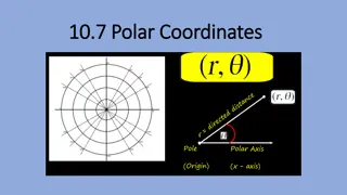
Understanding Polar Plots in System Analysis

The polar plot of a sinusoidal transfer function G(jω) represents the magnitude and phase angle of G(jω) on polar coordinates as ω varies from zero to infinity. It provides valuable insights into the frequency response characteristics of a system in a single plot. By following specific steps, you can draw a polar plot to analyze system behavior effectively, although it may not reveal individual factors' contributions.

Download Presentation

Please find below an Image/Link to download the presentation.
The content on the website is provided AS IS for your information and personal use only. It may not be sold, licensed, or shared on other websites without obtaining consent from the author. Download presentation by click this link. If you encounter any issues during the download, it is possible that the publisher has removed the file from their server.
E N D
Presentation Transcript
Introduction The polar plot of sinusoidal transfer function G(j ) is a plot of the magnitude of G(j ) verses the phase angle of G(j ) on polar coordinates as is varied from zero to infinity. Therefore it is the locus of as is varied from zero to infinity. As So it is the plot of vector as is varied from zero to infinity j j ( ) ( ) G G j j j = ( ) ( ) ( ) G G Me j ( ) Me
Introduction conti In the polar plot the magnitude of G(j ) is plotted as the distance from the origin while phase angle is measured from positive real axis. + angle is taken for anticlockwise direction. Polar plot is also known as Nyquist Plot. Adv: it depicts the frequency response characteristics over a the entire w in a single plot. Disadv: Plot does not indicate the contribution of each individual factor of the open loop transfer function.
Steps to draw Polar Plot Step 1: Determine the T.F G(s) Step 2: Put s=j in the G(s) Step 3: At =0 & = find by & Step 4: At =0 & = find by & Step 5: Rationalize the function G(j ) and separate the real and imaginary parts Step 6: Put Re [G(j ) ]=0, determine the frequency at which plot intersects the Im axis and calculate intersection value by putting the above calculated frequency in G(j ) lim lim j ( j ( j G ( ) G lim lim ) j G ( ) G 0 ) j j ( ) G ( ) G 0
Steps to draw Polar Plot conti Step 7: Put Im [G(j ) ]=0, determine the frequency at which plot intersects the real axis and calculate intersection value by putting the above calculated frequency in G(j ) Step 8: Sketch the Polar Plot with the help of above information
Polar plot of Type 0 system K s G + = ( ) Step 1: Put s=j 1 ( ) sT w M (in degrees) 0 -45 -90 w=0 M=1 w= M=0 0 1 1/T 0.707 0
Polar Plot for Type 0 System K Let = ( ) G s + + 1 ( )( 1 ) sT sT 1 2 Step 1: Put s=j K = ( ) G j + + 1 ( )( 1 K ) j T j T 1 2 = 1 1 tan tan T T ( ) ( ) 1 2 2 2 + + 1 1 T T 1 2 Step 2: Taking the limit for magnitude of G(j )
Type 0 system conti K lim = = ( ) G j K ( ) ( ) 2 2 + + 1 1 T j T 0 1 2 K lim = = ( ) 0 G j ( ) ( ) 2 2 + + 1 1 T j T 1 2 Step 3: Taking the limit of the Phase Angle of G(j ) lim = = 1 1 ( ) tan tan 0 G j T T 1 2 0 lim = = 180 1 1 ( ) tan tan G j T T 1 2
Type 0 system conti Step 4: Separate the real and Im part of G(j ) + + 2 1 ( ) ( ) K T T + K T T = ( ) 1 2 1 2 + G j j + + + 2 2 2 2 4 2 2 2 2 4 1 1 T T T T T T T T 1 2 1 2 1 2 1 2 Step 5: Put Re [G(j )]=0 1 ( + + T 2 ) K T T 1 = = = 1 2 0 & + 2 2 2 2 4 1 T T T T T 1 2 1 2 1 2 So When K T T 1 1 T 2 = j = 0 ( ) 90 G + T T T 1 2 1 2 = j = 0 & ( ) 0 180 G
Type 0 system conti Step 6: Put Im [G(j )]=0 K + T ( ) T T = = 0 0 & 1 2 + + When + 2 2 2 2 4 1 So T T T 1 2 1 2 = j = 0 0 ( ) 0 G K = j = 180 0 ( ) 0 G
Polar Plot for Type 1 System K Let = ( ) G s + + 1 ( s )( 1 ) sT sT 1 2 Step 1: Put s=j K = ( ) G j + + 1 ( )( 1 K ) j j T j T 1 2 = 90 tan tan 0 1 1 T T ( ) ( ) 1 2 + + 2 2 1 1 T j T 1 2
Type 1 system conti Step 2: Taking the limit for magnitude of G(j ) lim + K j G K = = ( ) G j ( ) ( ) 2 2 + 1 1 T j T 0 1 2 lim = = ( ) 0 ( ) ( ) 2 2 + + 1 1 T j T 1 2 Step 3: Taking the limit of the Phase Angle of G(j ) lim = = 0 1 1 0 ( ) 90 tan tan 90 G j T T 1 2 0 lim = = 270 0 1 1 0 ( ) 90 tan tan G j T T 1 2
Type 1 system conti Step 4: Separate the real and Im part of G(j ) + ( ) ( ) T 2 K T T + j K T T K = + ( ) G j j 1 2 1 2 + + + + + ( ) ( ) 3 2 2 2 2 2 3 2 2 2 2 2 T T T T T T T 1 2 1 2 1 2 1 2 Step 5: Put Re [G(j )]=0 T + ( ) K T T = = 1 2 0 So + at + + 3 2 2 2 2 2 ( ) T T T 1 2 1 2 = j = 0 ( ) 0 270 G
Type 1 system conti Step 6: Put Im [G(j )]=0 2 ( + + + T T ) T j K T T K 1 = = = 1 2 0 & 3 2 2 2 2 2 ( ) T T T 1 2 1 2 1 2 So When K T T 1 1 T 2 = j = 0 ( ) 0 G + T T T 1 2 1 2 = j = 0 ( ) 0 G
Polar Plot for Type 2 System K Let = ( ) G s + + 2 1 ( )( 1 ) s sT sT 1 2 Similar to above
Note: Introduction of additional pole in denominator contributes a constant -1800 to the angle of G(j ) for all frequencies. See the figure 1, 2 & 3 Figure 1+(-1800 Rotation)=figure 2 Figure 2+(-1800 Rotation)=figure 3
Ex: Sketch the polar plot for G(s)=20/s(s+1)(s+2) Solution: Step 1: Put s=j 20 + j = ( ) G j j j + ( 1 )( ) 2 20 + = 0 1 1 90 tan tan / 2 + 2 2 1 4
Step 2: Taking the limit for magnitude of G(j) 20 + lim j = = ( ) G + 2 2 1 4 0 20 + lim j = = ( ) 0 G + 2 2 1 4 Step 3: Taking the limit of the Phase Angle of G(j ) lim j = = 0 1 1 0 ( ) 90 tan tan / 2 90 G 0 lim = = 270 0 1 1 0 ( ) 90 tan tan / 2 G j
Step 4: Separate the real and Im part of G(j) 2 3 60 2 20 + ( 2 + ) j j = + ( ) G j + + 4 2 4 2 2 ( )( 4 ) ( )( 4 ) 2 60 = = 0 + + 4 2 2 ( So )( 4 ) at = j = 0 ( ) 0 270 G
Step 6: Put Im [G(j)]=0 3 20 + for ( 2 + ) j = = = 0 2 & 4 2 2 ( So )( 4 ) positive value of 10 = j = 0 2 ( ) 0 G 3 = j = 0 ( ) 0 0 G
Phase Crossover Frequency (p) : The frequency where a polar plot intersects the ve real axis is called phase crossover frequency Gain Crossover Frequency ( g) : The frequency where a polar plot intersects the unit circle is called gain crossover frequency So at g Unity j G = ) (
Phase Margin (PM): Phase margin is that amount of additional phase lag at the gain crossover frequency required to bring the system to the verge of instability (marginally stabile) m=1800+ Where = G(j g) if m>0 => +PM if m<0 => -PM (Stable System) (Unstable System)
Gain Margin (GM): ( j ) G The gain margin is the reciprocal of magnitude at the frequency at which the phase angle is -1800. In terms of dB 1 log 20 10 jwc G 1 1 = = GM | ( | ) G jwc x = = = 20 log | ( | ) 20 log ( ) GM in dB G jwc x 10 10 | ( | )
Stability Stable: If critical point (-1+j0) is within the plot as shown, Both GM & PM are +ve GM=20log10(1 /x) dB
Unstable: If critical point (-1+j0) is outside the plot as shown, Both GM & PM are -ve GM=20log10(1 /x) dB
Marginally Stable System: If critical point (-1+j0) is on the plot as shown, Both GM & PM are ZERO GM=20log10(1 /1)=0 dB
Inverse Polar Plot The inverse polar plot of G(j ) is a graph of 1/G(j ) as a function of . Ex: if G(j ) =1/j then 1/G(j )=j lim j = 1 ( ) 0 G 0 lim j = 1 ( ) G
Books Automatic Control system By S. Hasan Saeed Katson publication
Nyquist plot It gives information about both absolute stability and relative stability From Nyquist plot of open loop transfer function, relative stability of closed loop system can be obtained. We can find out frequency domain specifications. It is a graphical technique and does not require the exact determination of closed loop poles.
? ? ? ? =? ?+?1 ?+?2 . ?+?1 ?+?2 ., m<n ------(1) The characteristic equation is, q(s) = 1+ G(s)H(s) =0 ?+?1 ?+?2 +? ?+?1 ?+?2 . ?+?1 ?+?2 . q(s) = = 0 -----(2) q(s) = ? ?+?1 ?+?2 . ?+?1 ?+?2 . =o ---------(3) Poles of q(s) are poles of O.L.T.F. G(s)H(s) Zeros of q(s) are the roots of characteristic equation
For system to be stable, roots of ch eq must lie in LHS of S plane i.e. zeros of q(s) must lie in LHS of S plane. Zeros of ch eq are closed loop poles. If any of the zeros of q(s)lie in RHS, the system is unstable. The Nyquist stability criterion is based on the principle of argument. Principle of argument is related with theory of mapping.
Encirclement: Counting no of encirclement: A point is said to be encircled by a closed path if it is found to lie inside that closed path Anticlockwise dir as ref, N = 1 N = -2 N = 0
Theory of mapping Consider a function D(s)= s^2 +1 D(s) at s1 = 2+4j = ( 2+4j)^2+1 = -11+j16 S plane and D(s) plane We can say that every point in s plane maps into one and only one point in the D(s) plane.
Principle of argument/ Cauchys Principle
Principle of Argument Mapping theorem states that the mapped locus T (s) encircles the new origin of F plane as many times as the difference between the no of zeros and poles of F(s) which are encircled by T(s) path in s plane N = Z-P N = Encirclement of origin of F plane P , Z= No of poles and zeros of F(s) encircled by T(s) path in s plane Remember from the Cauchy criterion that the number N of times that the plot of G(s)H(s) encircles -1 is equal to the number Z of zeros of 1 + G(s)H(s) enclosed by the frequency contour minus the number P of poles of 1 + G(s)H(s) enclosed by the frequency contour (N = Z - P).
The Nyquist Stability Criterion Poles of 1+G(s)H(s) = poles of G(s)H(s)= open loop poles Zeroes of 1+G(s)H(s)= closed loop poles of system For stability all the zeros of 1+G(s)H(s) must be in LHS, none of the zeros must in RHS Nyquist suggested that rather than analyzing whether all the zeroes are located in LHS, it is better to locate the presence of ant zero of 1+G(s)H(s) in RHS making the system unstable. So active region is RHS. He suggested a contour which will encircle the RHS S = +j to s= -j Nyquist path
The Nyquist Stability Criterion The Nyquist plot allows us also to predict the stability and performance of a closed-loop system by observing its open-loop behavior. The Nyquist criterion can be used for design purposes regardless of open-loop stability (Bode design methods assume that the system is stable in open loop). Therefore, we use this criterion to determine closed-loop stability when the Bode plots display confusing information. The Nyquist diagram is basically a plot of G(j* w) where G(s) is the open-loop transfer function and w is a vector of frequencies which encloses the entire right-half plane. In drawing the Nyquist diagram, both positive and negative frequencies (from zero to infinity) are taken into account. In the illustration below we represent positive frequencies in red and negative frequencies in green. The frequency vector used in plotting the Nyquist diagram usually looks like this (if you can imagine the plot stretching out to infinity): However, if we have open-loop poles or zeros on the jw axis, G(s) will not be defined at those points, and we must loop around them when we are plotting the contour. Such a contour would look as follows:R tends to
The Cauchy criterion The Cauchy criterion (from complex analysis) states that when taking a closed contour in the complex plane, and mapping it through a complex function G(s), the number of times that the plot of G(s) encircles the origin is equal to the number of zeros of G(s) enclosed by the frequency contour minus the number of poles of G(s) enclosed by the frequency contour. Encirclements of the origin are counted as positive if they are in the same direction as the original closed contour or negative if they are in the opposite direction. When studying feedback controls, we are not as interested in G(s) as in the closed-loop transfer function: G(s) --------- 1 + G(s) If 1+ G(s) encircles the origin, then G(s) will enclose the point -1. Since we are interested in the closed-loop stability, we want to know if there are any closed-loop poles (zeros of 1 + G(s)) in the right-half plane. Therefore, the behavior of the Nyquist diagram around the -1 point in the real axis is very important; however, the axis on the standard nyquist diagram might make it hard to see what's happening around this point
Gain and Phase Margin Gain Margin is defined as the change in open-loop gain expressed in decibels (dB), required at 180 degrees of phase shift to make the system unstable. First of all, let's say that we have a system that is stable if there are no Nyquist encirclements of -1, such as : 50 ----------------------- s^3 + 9 s^2 + 30 s + 40 Looking at the roots, we find that we have no open loop poles in the right half plane and therefore no closed-loop poles in the right half plane if there are no Nyquist encirclements of -1. Now, how much can we vary the gain before this system becomes unstable in closed loop? The open-loop system represented by this plot will become unstable in closed loop if the gain is increased past a certain boundary.
Gain and Phase Margin Phase margin as the change in open-loop phase shift required at unity gain to make a closed-loop system unstable. From our previous example we know that this particular system will be unstable in closed loop if the Nyquist diagram encircles the -1 point. However, we must also realize that if the diagram is shifted by theta degrees, it will then touch the -1 point at the negative real axis, making the system marginally stable in closed loop. Therefore, the angle required to make this system marginally stable in closed loop is called the phase margin (measured in degrees). In order to find the point we measure this angle from, we draw a circle with radius of 1, find the point in the Nyquist diagram with a magnitude of 1 (gain of zero dB), and measure the phase shift needed for this point to be at an angle of 180 deg.
Consider the Negative Feedback System Remember from the Cauchy criterion that the number N of times that the plot of G(s)H(s) encircles -1 is equal to the number Z of zeros of 1 + G(s)H(s) enclosed by the frequency contour minus the number P of poles of 1 + G(s)H(s) enclosed by the frequency contour (N = Z - P). Keeping careful track of open- and closed-loop transfer functions, as well as numerators and denominators, you should convince yourself that: the zeros of 1 + G(s)H(s) are the poles of the closed-loop transfer function the poles of 1 + G(s)H(s) are the poles of the open-loop transfer function. The Nyquist criterion then states that: P = the number of open-loop (unstable) poles of G(s)H(s) N = the number of times the Nyquist diagram encircles -1 clockwise encirclements of -1 count as positive encirclements counter-clockwise (or anti-clockwise) encirclements of -1 count as negative encirclements Z = the number of right half-plane (positive, real) poles of the closed-loop system The important equation which relates these three quantities is: Z = P + N
The Nyquist Stability Criterion - Application Knowing the number of right-half plane (unstable) poles in open loop (P), and the number of encirclements of -1 made by the Nyquist diagram (N), we can determine the closed-loop stability of the system. If Z = P + N is a positive, nonzero number, the closed-loop system is unstable. We can also use the Nyquist diagram to find the range of gains for a closed-loop unity feedback system to be stable. The system we will test looks like this: where G(s) is : s^2 + 10 s + 24 --------------- s^2 - 8 s + 15
The Nyquist Stability Criterion This system has a gain K which can be varied in order to modify the response of the closed-loop system. However, we will see that we can only vary this gain within certain limits, since we have to make sure that our closed-loop system will be stable. This is what we will be looking for: the range of gains that will make this system stable in the closed loop. The first thing we need to do is find the number of positive real poles in our open-loop transfer function: roots([1 -8 15]) ans = 5 3 The poles of the open-loop transfer function are both positive. Therefore, we need two anti- clockwise (N = -2) encirclements of the Nyquist diagram in order to have a stable closed-loop system (Z = P + N). If the number of encirclements is less than two or the encirclements are not anti-clockwise, our system will be unstable. Let's look at our Nyquist diagram for a gain of 1: nyquist([ 1 10 24], [ 1 -8 15]) There are two anti-clockwise encirclements of -1. Therefore, the system is stable for a gain of 1.
The Nyquist Stability Criterion MathCAD Implementation = 100 99.9 = = j w w 100 j 1 s w ( ) ( )2 + 10 s w + s w ( )2 ( ) 24 = G w ( ) There are two anti- clockwise encirclements of -1. Therefore, the system is stable for a gain of 1. 8 s w + s w ( ) 15 2 Im G w ( ( ) ) 0 0 2 2 1 0 1 2 Re G w ( ( ) )


=20/s(s+1)(s+2)")
")
")
]=0")
]=0")

 : The frequency where a")
:")
:")

 is outside the plot")
 is")