Understanding Root Locus Plots for Control Systems

Exploring the concept of root locus plots in control systems through a detailed analysis of feedback systems, rise time optimization, steady-state errors, and closed-loop response predictions. The content discusses the impact of varying proportional gain on system performance, practical examples from cruise control systems, and the interpretation of root locus plots to predict system behavior.

• Control systems
• Root locus plots
• Feedback analysis
• System optimization
• Closed-loop response

kays_498 Follow

Uploaded on Sep 17, 2024 | 0 Views

Download Presentation

Please find below an Image/Link to download the presentation.

The content on the website is provided AS IS for your information and personal use only. It may not be sold, licensed, or shared on other websites without obtaining consent from the author. Download presentation by click this link. If you encounter any issues during the download, it is possible that the publisher has removed the file from their server.

Presentation Transcript

1. 01/17/19

2. 01/17/19

3. 01/17/19

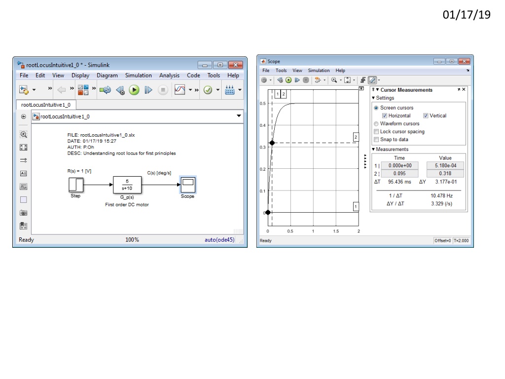
4. 01/17/19 \labviewCourseDevelopment\labview=0X-RootLocus\pptRootLocusNotesAndFigures011719.pptx Michigan reference: Cruise Control example http://ctms.engin.umich.edu/CTMS/index.php?example=CruiseControl&section=ControlRootLocus Reference ? ? set for 10 m/s, so want car speed ? ?to be 10 m/s so need to increase ?? ??= 25 ???= 5;??= 19.7 sec ??= 50 ???= 10;??= 19.7 sec

5. 01/17/19 What happens when have (unit) feedback? ???= 5;??= 9.8 sec (with feedback) vs. 19.7 sec (just open-loop). Rise time improves! ??= 50but with simply fed back the car s speed ??= 5000 ???= 9.89.;??= 0.215 sec ???= 8;??= 4.02 sec ??= 200

6. 01/17/19 Observations of feedback: Increasing (proportional) gain ?? gets us closer to desired car speed ?(?)??= 10 m/s Increasing ?? reduces rise time ?? However, even with ??= 5000, we have a steady-state error (this is because the plant is a Type 0 system Wouldn t be great if we can predict what the (closed-loop feedback) output would be (i.e. ?(?)??) given different values of ??? This is what the root locus plot does ? ? = ? ? ????? = ????(?) ? ? ?(?)?(?) ??(?) ? ? ?(?) + ????? = ????? ?(?) ????(?) ?(?) + ????? Hence:?(?) Is the equivalent TF ?(?)= ?(?) ? ? ????(?) ?(?) + ????? 1 ?? The characteristic equation is the roots of the denominator i.e. ?(?) + ????? = 0 ?? 1000? + 50 = 1 1000? + 50 + ?? 1 + ?? 1000? + 50 Note to self: when s=0 and take limit, we see steady- state response matches of the graphs in previous slide

7. 01/17/19 1000? + 50=1000? + 50 + ?? 1 1 + ????? = 0 1 + ?? = 0 1000? + 50 Next time: Not sure how the above RL helps us predict response i.e. if trace along the loci for a gain, say near 200, we still don t know the output value

8. 01/17/19 How does the above values from the RL (left) correspond to output response (right)? Observe that 1 1 ?= 0.25= 4(which is the rise time on the left) ????(?) 1+?????= lim ? 0 Note to self: Should be 8, not 0.8 missing something ?? 200 We also have lim 1000?+50+??= 50+200= 0.8 ? 0

9. 01/19/19 Recall from 01/17/19, that with (unity) feedback, we can (almost) get to the desired steady- state response ???= 9.89.;??= 0.215 sec ??= 5000 Recall from 01/17/19, that the CLTF for the above block diagram was 1 ?? ????(?) ?(?) + ????? ?(?) ?(?)= ?? ?(?) ?(?)= 1000? + 50 = Or 1 1000? + 50 + ?? 1 + ?? 1000? + 50

10. 01/19/19 If we have step input ? ? ?? ? (recall that command is 10 m/s) then have ?? ?? ? ? = 1000? + 50 + ?? ? But recall that Final Value Theorem says that ? ? |??= lim ? ?(?) lim ? 0??(?) ?? 10 1000? + 50 + ?? ?? 10 50 + ?? 1 ? ? |??= lim ? 0??(?) = lim ? 0? ?= Thus for our case, we have Recall (previous slide and from 01/17/19), that for ?? 5000 we had ? ? |??= 9.89 5000 10 50 + 5000= 9.90 ? ? |??= Which is the same, thus QED For this particular case (?? 5000) the CLTF is ?? ?(?) ?(?)= 5000 = 1000? + 50 + ?? 1000? + 50 + 5000 ? = 5050 1000 So, the CLTF pole is = 5.05

11. 01/19/19 Sadly, Matlab would not display the Gain above 4000. However, one sees that the pole value is converging to the calculated value. To fully convince ourselves, recall that 01/17/19 we showed that ?? 200 as below The resulting CLTF would be ?? ?(?) ?(?)= 200 = 1000? + 50 + ?? 1000? + 50 + 200 ? = 250 1000= 0.25 So, the CLTF pole is Thus QED We also see for ?? 200 that the steady-state would be ?? 10 50 + ?? = 8 Thus QED 200 10 50 + 200=2000 ? ? |??= = 250

12. 01/19/19 Thus far, we see the following: (Unity) Feedback on a proportional gain (??) plant (??(?)) has shorter rise time For Type 0 system (like this case), step input results in a steady-state error The gain might need to be very high to achieve the desired output It s unclear if one can physically implement such a high gain Lag control attempts to improve steady-state response. So, we can try to eliminate the steady-state error. For our current design system, say ?? 200, the error is quite high (10 m/s 8 m/s = 2 m/s) Let s try to reduce this error by a 100th, i.e. we can live with 0.02 m/s of error ? +1 ? +1 ?? + 1 ??? + 1= ?? ? ??? ??? where ??: Gain of the lag compensator ?? Note to self: I believe that to reduce the error by a 100th, one sets ? 100 Next time: Try to create and test a lag compensator with the above equation and ?

13. 01/22/19 Recall from 01/19/19 that for ?? 200, the steady-state error = 2 m/s Let s try to reduce this error by a 10th, i.e. we can live with 0.2 m/s of error ? +1 ? +1 ?? + 1 ??? + 1= ?? ? where ??: Gain of the lag compensator ??? ??? ?? To reduce the error by a 10th, one sets ? 10 and one has pole and zero near origin, so try: ? +1 0.5 1 ?0.5 ? + 2 ? +1 ? + 2 ? + 0.2 ??? ?? = ?? = ?? Observe: ???= 0.26 m/s which is what we designed for ? + 5

14. 01/22/19 Uncompensated system (01/19/19) Lag Compensated system (01/22/19) ???= 8.0;??= 4.020 sec with ?? 200 ???= 9.74;??= 1.721 sec with ?? 200 Contrasting the above, we see that Lag Compensation introduces overshoot (and a shorter rise-time). This makes sense because Lag is like a ?+0.2 1 1 ? integrator. Q1: Can one change ??from 1 to another value, to reduce overshoot? Next time: show RL for the lag compensated opened loop transfer function

15. 01/23/19 Goal: Plot Root Locus of the following: ??(?) ??(?) ? ? = ????????? = ????????? ?? ?(?) 1 But say that ? ? 1 + ???????? = ?????????(?) ?? + ? ? + ? 1 + ?? + ? 1 ???????? 1 + ???????? ?(?) ?(?)= ?(?) ?(?)= 1000? + 50 Where ? ???? 1 ? + ? 1000? + 50 ?(?) ?(?)= ?(? + ?) This would be the opened loop TF ??(?) ? + ? 1000? + 50 + ?(? + ?) Note to self: I think the above might be wrong see my ogataExample7.2-Notes-011419a.pptx

16. 01/23/19 Using Ogata Example 7-2 (pg. 420) as guidance R(s) ??(?) 1 + ??? ?(?) ?(?)= ?(?) ?(?) ? ? ??(?) 1 + ??? 1 1 1000? + 50 = 1 1000? + 50 + 1 1 + 1000? + 50 Lag Compensated System is: ??(?) ??(?) ? + ? ? + ? ??? = ?? Where ? = 2 and ? = 0.2 ? + ? ? + ? 1 ? + 2 ? + 0.2 1 ??? ? ? = ?? 1000? + 51= ? 1000? + 51 Plot the RL of this

17. 01/23/19 Looks like the same on U Michigan Cruise Control site (with zero = 0.3 and pole = 0.03 Next time: try things like sgrid(0.6, 0.36) and using the rlocfind command again

18. 01/23/19

19. 01/23/19

20. 01/23/19