Visualising and Exploring BS-Seq Data: Tips and Insights
Explore essential strategies for analysing BS-Seq data, ranging from selecting appropriate methylation contexts to identifying coverage outliers and biases. Understand how to interpret data patterns, handle unusual findings, and mitigate potential errors, ensuring accurate methylation analysis results.

Download Presentation

Please find below an Image/Link to download the presentation.
The content on the website is provided AS IS for your information and personal use only. It may not be sold, licensed, or shared on other websites without obtaining consent from the author.If you encounter any issues during the download, it is possible that the publisher has removed the file from their server.
You are allowed to download the files provided on this website for personal or commercial use, subject to the condition that they are used lawfully. All files are the property of their respective owners.
The content on the website is provided AS IS for your information and personal use only. It may not be sold, licensed, or shared on other websites without obtaining consent from the author.
E N D
Presentation Transcript
Visualising and Exploring BS-Seq Data Simon Andrews simon.andrews@babraham.ac.uk @simon_andrews v2021-04
Starting Data Read 1 Read 2 Read 3 Genome L001_bismark_bt2_pe.deduplicated.bam CHG_OB_L001_bismark_bt2_pe.deduplicated.txt.gz CHG_OT_L001_bismark_bt2_pe.deduplicated.txt.gz CHH_OB_L001_bismark_bt2_pe.deduplicated.txt.gz CHH_OT_L001_bismark_bt2_pe.deduplicated.txt.gz CpG_OB_L001_bismark_bt2_pe.deduplicated.txt.gz CpG_OT_L001_bismark_bt2_pe.deduplicated.txt.gz L001_bismark_bt2_pe.deduplicated.cov.gz
Decide early on which data to use Methylation contexts CpG: Only generally relevant context for mammals CHG: Only known to be relevant in plants CHH: Generally unmethylated Methylation strands CpG methylation is generally symmetric Normally makes sense to merge OT / OB strands
Always start by looking at your data. Think about what you expect Reads (red=for blue=rev) Calls (red=meth blue=unmeth)
Try to understand anything unusual Very messed up cDNA contaminated library
Try to understand anything unusual Around 600x average genome density Coverage Outliers
Coverage Outliers Normally the result of mis-mapping repetitive sequences not in the genome assembly Centromeric / telomeric sequences are common Can be a significant proportion of all data Can throw off calculations of overall methylation Should be flagged and hits in those regions ignored
Coverage Bias GC Content is most likely but others could exist
Where to make measures Per base Very large number of measures Poor accuracy for individual bases Unbiased windows Tiled over whole genome Need to decide how they will be defined Targeted regions Which regions What context
Accuracy and Power Region A Region B 50% Methylation 50% Methylation Variation in CpG density Variation in coverage depth
Try to make comparable measures Observation level correlates with stability. Want to try to have similar amounts of data in each measurement window. Equalises noise for visualisation and power for analysis.
Unbiased Analysis Fix the amount of data in each window Fixed number of CpGs per window Allow the resolution to vary 50 CpG window lengths
Targeted Quantitation Measure over features CpG islands Be careful where you get your locations Try to fix sizes Promoters Should probably split into CpG island and non-CpG island Try to fix sizes Gene bodies Filter by biotype to remove small RNA genes?
How to Quantitate methylation calls Percentage methylation (Methylated calls / Total Calls) * 100 = meth = unmeth (6/10) * 100 = 60% methylated
Assigning a % methylation value to a region can be difficult. Total methylated calls = 15 Total unmethylated calls = 10 Methylation level = (15/(15+10))*100 = 60%
You get different answers quantitating per base or per region Percentage methylation from all calls independently = 46% Percentage methylation from mean methylation per base = 80%
Coverage differences can look like methylation differences 67% 43% Common = 60% in both
Coverage differences arent just a theoretical concern they affect real data p=3.2-7
Coverage differences arent just a theoretical concern they affect real data 47% 94%
Levels of Complexity Simple Percentage of all calls which are methylated Per base methylation, averaged over a region Bases excluded because of low coverage As above, but requiring the same bases to be used in each sample Doesn't scale well Complex
(Even) More Complex Methods Smoothing or regression of actual measures along a chromosome. Aims to reduce noise from sampling variation Relies on consistent linear patterns Imputation of missing values Relies on consistent linear patterns Additional normalisation or correction Will be discussed later
Use visualisation to understand the basic structure of your data before asking questions Patterning What sorts of changes in methylation do I observe along a chromosome Distributions What are the overall levels and distributions of methylation values in my samples Relationships On a global scale what is the overall relationship between methylation levels in different conditions
Visualise your quantitated data alongside the raw methylation calls.
Different representations scale to different numbers of samples.
Understand and compare your methylation distributions before formulating a question.
Plotting comparisons will identify global differences which might be interesting
Look at the data underneath and around potentially interesting points
Large global changes might mean that local analysis is no longer relevant
Small differences in distribution can be normalised to improve comparisons
Trend Plots Effects at individual loci can be subtle Want to find more generalised effect Collate information across whole genome Look at the general trends Relies on the effect being consistent
Trend plot considerations Axis Scaling What measures How much context Features to use How much context
Clustering Correlation Clustering Focusses on the differences between conditions Absolute values not important Look for similar trends Show median normalised values Euclidean Clustering Focusses on absolute differences between conditions Look for similar levels Show raw values
Clustering Euclidean Clustering Correlation Clustering
Exploration Summary (1) Look at the distribution of your raw reads/calls Do they match what you expect from the library type? Always start with an unbiased quantitation Fix the amount of data in each window Think about how to best quantitate Check the quantitation matches the raw data
Exploration Summary (2) Check the distributions of methylation values in your samples Are there big differences between your samples? Directly compare your values to look for global differences They might be the source of the interesting biology Might spot small global differences which require normalisation Summarise trends around features Might justify targeted quantitation


 More Complex Methods")


")
")