Variance Estimation in Social Surveys: Using R for Complex Sampling
Explore the importance of social surveys in capturing key indicators like employment rates, spending, and wealth through a multistage sampling design. Learn about variance estimation in complex surveys, calibration techniques, and the linearised jackknife method for analyzing survey data. Discover the history of implementations in the ONS and the rise of R for survey data analysis.
Download Presentation

Please find below an Image/Link to download the presentation.
The content on the website is provided AS IS for your information and personal use only. It may not be sold, licensed, or shared on other websites without obtaining consent from the author.If you encounter any issues during the download, it is possible that the publisher has removed the file from their server.
You are allowed to download the files provided on this website for personal or commercial use, subject to the condition that they are used lawfully. All files are the property of their respective owners.
The content on the website is provided AS IS for your information and personal use only. It may not be sold, licensed, or shared on other websites without obtaining consent from the author.
E N D
Presentation Transcript
Using R for variance estimation in social surveys Eleanor Law and Vah Nafilyan, ONS
Social surveys Crucial for key indicators: Employment and unemployment rates (Labour Force Survey) Spending (Living Costs and Food Survey) Pension/financial/property wealth (Wealth and Assets Survey) Many more! Sampling frame is usually the postcode address file (PAF)
Complex sample design Multistage sampling e.g. WAS Primary sampling unit is a postcode sector Systematic sampling after ordering by social demographic indicator/car ownership Image credit: http://researchhubs.com/post/ai/data-analysis-and-statistical- inference/observational-studies-and-experiments-sampling-and-source-bias.html
Calibration Limited control over the make up of the sample Non-response rates differ between different groups Weighting can compensate for over/underrepresentation of sex/age/region groups in the sample Calibration can reduce standard error of estimates if poststrata correlate with variable of interest
Variance in complex surveys Established formulae for calculation of variance, accounting for strata and clustering Implemented in the R survey package These do not consider the effect of calibration
The linearised jackknife Fitting a linear model for the variable of interest as a function of the poststrata This establishes how much of the variance is accounted for by the poststrata as explanatory variables Variance that exists in the residuals, after the poststrata have been accounted for, is what we want to know
History of implementations in ONS Lots of existing weighting code for a range of surveys Widely used across ONS in business areas Holmes & Skinner for LFS Generic STATA SAS 2000 2005 2010 2015 R Free and open source! Increasing use of R and python across ONS
Developing a package Standard formatting for R packages Automatically generated documentation: library(devtools) load_all("D:/glinjack_git/Glinjack/glinjack") document("D:/glinjack_git/Glinjack/glinjack") User-friendly focus in definition of arguments
Reproducing standard errors - APS Personal well-being in the UK Calibration to age X sex, local authorities Four well-being variables: Life satisfaction, happiness, sense of worthwhileness and anxiety Estimates of average and percentage with very high/high/medium/low levels Estimates by age, gender, country and local authority Very time consuming in SAS
Computational efficiency APS personal well being (headline estimates) WAS mean physical wealth (1) WAS total estimates (6) SAS 1320 11 15 R 40 2 8
Variance estimation for households Poststrata are usually either One categorical variable OR Split into dummy binary variables Household level data are aggregated: Region Region Sex/age group 1 Sex/age group 2 Sex/age group 3 1 0 0 0 0 2 1 1 1 3 Person 1 Person 2 Person 3 Household total 0 1 0 1 0 0 0 0 1 0 1 2
Reproducing standard errors - WAS Wave 5 (2014-2016) estimates of total/financial/property/physical wealth etc Standard Errors originally calculated in SAS Quality assured by reproduction using R This highlighted a problem with the parameter definitions passed to the SAS macro
Reproducing standard errors - WAS Waves 3-5 (2010-2016) estimates of the percentage of dependent children in households with problem debt Originally calculated in SAS Attempted reproduction using R Very similar, but not identical, results obtained, indicating there was a slight methodological difference SAS method aggregates members of a household before calculating residuals
Future Developments Further testing including collaboration to get user feedback Ratio estimates for domains Aggregation over households within the R function Variance of change Very similar method, using input of two datasets Could be combined with glinjack into one R function and package
Acknowledgements Ria Sanderson SD&E(S) team
