Understanding Toeplitz Matrix 1x1 Convolution in Deep Learning
Explore the concept of Toeplitz Matrix 1x1 Convolution in deep learning for processing arbitrary-sized images. Discover how this technique enables running ConvNets on images of various dimensions efficiently, making use of matrix multiplication with Toeplitz matrices to achieve convolution. Dive into the importance and applications of Toeplitz matrices in convolutional neural networks and grasp the fundamentals through insightful visuals and explanations.
Download Presentation

Please find below an Image/Link to download the presentation.
The content on the website is provided AS IS for your information and personal use only. It may not be sold, licensed, or shared on other websites without obtaining consent from the author. Download presentation by click this link. If you encounter any issues during the download, it is possible that the publisher has removed the file from their server.
E N D
Presentation Transcript
ECE 6504: Deep Learning for Perception Topics: Toeplitz Matrix 1x1 Convolution AKA How to run a ConvNet on arbitrary sized images Dhruv Batra Virginia Tech
Plan for Today Toeplitz Matrix 1x1 Convolution AKA How to run a ConvNet on arbitrary sized images (C) Dhruv Batra 2
Toeplitz Matrix Diagonals are constants Aij = ai-j (C) Dhruv Batra 3
Why do we care? (Discrete) Convolution = Matrix Multiplication with Toeplitz Matrices (C) Dhruv Batra 4
"Convolution of box signal with itself2" by Convolution_of_box_signal_with_itself.gif: Brian Ambergderivative work: Tinos (talk) - Convolution_of_box_signal_with_itself.gif. Licensed under CC BY-SA 3.0 via Commons - https://commons.wikimedia.org/wiki/File:Convolution_of_box_signal_with_itself2.gif#/media/File:Convolution_of_box_signal_wi th_itself2.gif (C) Dhruv Batra 5
Why do we care? Two way of writing the same thing (C) Dhruv Batra 6
Plan for Today Toeplitz Matrix 1x1 Convolution AKA How to run a ConvNet on arbitrary sized images (C) Dhruv Batra 7
Convolutional Nets a C3: f. maps 16@10x10 C1: feature maps 6@28x28 S4: f. maps 16@5x5 INPUT 32x32 S2: f. maps 6@14x14 C5: layer 120 OUTPUT 10 F6: layer 84 Gaussian connections Full connection Subsampling Subsampling Full connection Convolutions Convolutions (C) Dhruv Batra Image Credit: Yann LeCun, Kevin Murphy 8
Classical View (C) Dhruv Batra 9 Figure Credit: [Long, Shelhamer, Darrell CVPR15]
Classical View = Inefficient (C) Dhruv Batra 10
Classical View (C) Dhruv Batra 11 Figure Credit: [Long, Shelhamer, Darrell CVPR15]
Re-interpretation Just squint a little! (C) Dhruv Batra 12 Figure Credit: [Long, Shelhamer, Darrell CVPR15]
Fully Convolutional Networks Can run on an image of any size! (C) Dhruv Batra 13 Figure Credit: [Long, Shelhamer, Darrell CVPR15]
Fully Convolutional Networks Up-sample to get segmentation maps (C) Dhruv Batra 14 Figure Credit: [Long, Shelhamer, Darrell CVPR15]
Note: After several stages of convolution-pooling, the spatial resolution is greatly reduced (usually to about 5x5) and the number of feature maps is large (several hundreds depending on the application). It would not make sense to convolve again (there is no translation invariance and support is too small). Everything is vectorized and fed into several fully connected layers. If the input of the fully connected layers is of size Nx5x5, the first fully connected layer can be seen as a conv. layer with 5x5 kernels. The next fully connected layer can be seen as a conv. layer with 1x1 kernels. (C) Dhruv Batra 15 Slide Credit: Marc'Aurelio Ranzato
H hidden units / Hx1x1 feature maps NxMxM, M small Fully conn. layer / Conv. layer (H kernels of size NxMxM) (C) Dhruv Batra 16 Slide Credit: Marc'Aurelio Ranzato
K hidden units / Kx1x1 feature maps H hidden units / Hx1x1 feature maps NxMxM, M small Fully conn. layer / Conv. layer (H kernels of size NxMxM) Fully conn. layer / Conv. layer (K kernels of size Hx1x1) Slide Credit: Marc'Aurelio Ranzato (C) Dhruv Batra 17
Viewing fully connected layers as convolutional layers enables efficient use of convnets on bigger images (no need to slide windows but unroll network over space as needed to re-use computation). TRAINING TIME Input CNN Image TEST TIME Input Input CNN Image Image y x (C) Dhruv Batra 18 Slide Credit: Marc'Aurelio Ranzato
Viewing fully connected layers as convolutional layers enables efficient use of convnets on bigger images (no need to slide windows but unroll network over space as needed to re-use computation). TRAINING TIME Input CNN Image CNNs work on any image size! TEST TIME Input CNN Image y x Unrolling is order of magnitudes more eficient than sliding windows! Slide Credit: Marc'Aurelio Ranzato (C) Dhruv Batra 19
Benefit of this thinking Mathematically elegant Efficiency Can run network on arbitrary image Without multiple crops Dimensionality Reduction! Can use 1x1 convolutions to reduce feature maps (C) Dhruv Batra 20
