Exploring Anomalies in Realistic Global Flows Using Matrix Physics
Investigate how matrix physics can provide a novel approach in understanding global climate models, focusing on realistic global flows and anomalies. The study aims to move beyond traditional algorithmic rule sets, examining how deviations from time mean flows can affect climate and weather patterns. Implementing a unique matrix calculation method, the research isolates variability to improve our understanding of climate dynamics and model accuracy.
Download Presentation

Please find below an Image/Link to download the presentation.
The content on the website is provided AS IS for your information and personal use only. It may not be sold, licensed, or shared on other websites without obtaining consent from the author. Download presentation by click this link. If you encounter any issues during the download, it is possible that the publisher has removed the file from their server.
E N D
Presentation Transcript
Matrix "anomaly physics" in realistic global flows Brian Mapes, Patrick Kelly, Siwon Song RSMAS, University of Miami
Motivation Most GCM physics schemes are algorithmic rule sets, defined in mathematical frameworks based in conceptual cartoons (idealizations). 1. Possibilities are countless...we could fiddle forever, neither understanding quite how our "reasonable" assumptions really play out, nor covering a bounded space of possibilities. 2. Impacts on mean state (climate) & fluctuations (weather) are entangled, muddling MJO esp.
Our Approach: Let's cast physics as a Matrix calculation 1. A finite, well-defined space of coefficients linking tendencies to state variables in an air column. locally linearized -- like Calculus, and that's quite general... 2. Isolate variability: make anomalous tendencies (deviations from a time mean) in realistic time-mean flow maintained by calibrated, time-independent forcing (the climatology of nudging, measured from nudged runs)
The background global model A Dry PE solver with time-independent, 3D forcing (sources-sinks) of T, q, div, vort forcing represents the time mean of all physics including fluxes by missing scales of motion and compensations for numerics errors devised to give realistic climatology for a particular resolution and viscosity for a particular season here perpetual JJA or OND following: Hall (2000), Lin Brunet & Derome (2007), Sardeshmukh and Sura (2009), Leroux Kiladis Hall (2011), ...
First model: simple and cheap 5 levels (900,700,500,300,100 mb). deep convection only touches the first 4 Four internal vertical modes Low res = R15 today Dry-run variability comes from hydrodynamic instabilities only
Model's discrete dry wave spectrum (4 internal modes, as tickled by dry hydrodynamic instabilities) wave7/1d = 66 m/s wave7/1d = 66 m/s 33 33 10 10
Quiz 1: on dry general circulation 1. We first nudged the model to climatological averaged JJA flow (u,v,T). this suppresses transients, as well as enforcing closeness to the observed large-scale mean state 2. In second run, the time mean of this nudging is used as a time-invariant forcing. transients now occur due to shear instabilities Can you guess how the mean flow differs from observed climo, due to dry transient eddy-mean flow interaction?
Quiz 1: on dry general circulation Answer in Patrick's talk (Part II). Stay awake.
"Dry" model also has a tracer q model includes tracer q: Dq/Dt = Sq(x,y,p) Sq devised to give water vapor-like climatology but q is unbounded Negative Sq regions can create q<0 no Clausius equation yet to limit positives
Quiz 2: "Dry" model with tracer q Dry-transient driven mean flow errors (see Quiz 1) advect q Can you guess what happens to the JJA Asian monsoon (as seen in PW for example)?
Ready for Matrix physics: X/ t|phy = MX But what state vector X? & what matrix M? Is it "linear"? Depends what you mean. M (x,y?,t?,U?,T?,q?,(P-E)?,?)
X/t = MX If the time-invariant forcing is devised to be correct time-mean physical tendencies, which give a realistic time-mean state, then our matrix outputs should be intended to act as anomalous physical tendencies that is, deviations from the time mean
X/t = MX How to get anomalous physical tendencies? If the inputs Xare anomalies, and M is time independent, then outputs MX(tendencies) will likewise be anomalies because any linear combination of zero-mean input variables also has zero mean
State vector X : a possible choice T' profile for matrix-based convection using Kuang (2010)'s CRM-derived M q' profile Windspeed' for WISHE, shear' for CRF... ...(Or whole u' profile for CMT)... ...
shear dep. anvil CRF hum. dep. anvil CRF WIS HE "Moist Convection": Each matrix column in this section adjusted to conserve MSE MSE sources WIS ME Surface ...& on shear CMT depends on C (thus on T',q')... friction
shear dep. anvil CRF WIS HE A space for estimation "Moist Convection": Each matrix column in this section conserves MSE (serious work)... WIS ME and postulation (incisive play)! Sfc. ...& on shear CMT depends on C (thus on T',q')... friction
As linear (or not) as you want... M a global constant very linear math system whatever it does can be analytically deconstructed clipping of hydrologic negatives, extremes, etc. physically possible; difference from above interesting (bias) M devised very locally in space, time, regime you can build in any relationship you think you know...
So far, we only show... Thermo. physics
So far, we only show... MSE-conserving moist convection matrix Mc
Anomaly physics 1: MSE conserving Anomalous moist convection represents anomalous condensation + vertical eddy flux divergences Scaled by clim. rainrate (e.g. zero where no rain) Kuang (2010) devised a clever way to estimate Mc, from interrogation of a periodic, partly-disabled CRM (no radiation, ...), via matrix inversion exploiting surprising linearizability also noted in Tulich and Mapes (JAS, 2010, same issue as Kuang)
Time scale of desired response: GCM timestep? (no, timescale implied by scale separations...) M instantaneous tendency etc. largely local diffusion We want convection's responses integrated over a deep cloud system life cycle say 4h
Friendlier "plot view" of the quadrants of M4h (published in Kuang 2012 JAS) Heat source sensitivities: Moisture source sensitivities:
Enhancement of deep convection by q' at any level Inhibition of deep convection by T' in 500-850mb Heat source sensitivities: PBL T or q good for deep conv (CAPE) Moisture source sensitivities:
Eyeball regrid to 900,700,500,300 then MSE balancing, then eigenvalue negation for stability Heat source sensitivities: Moisture source sensitivities:
Still has T700 inhibition and q700 sens. Heat source sensitivities: Moisture source sensitivities:
EXPERIMENT: set this column to 0 Heat source sensitivities: Moisture source sensitivities:
SUMMARY OF FORMULATION Bias-correct a "bad" GCM (here a dry PE solver) by turning climatology of nudging-to-obs into a time- independent forcing good mean flow A time-independent (but clim. rain scaled) M times an anomaly state vector anomaly tendencies coupled w/ global dyn. interesting (unforeseeable) Postulations in M space nice clean expts e.g. How does tropical weather depend on convection's FT moisture sensitivity ( convection/ q700)? ...on MSE sources ( Fsfc/ ', CRF/ ')? Moist transients that result may lead to noise- induced climate drift but that is interesting too...
Patrick's challenge He will show our/his very very first results... We will do several things differently next time! (Like next week! But not today...deadline-fresh results...) 1. We nudged to climatology, not obs w/ eddies Quiz: what happens to our JJA monsoon in no-M case? 2. Only 5 levels (4 int. modes for M to couple to) Unknown discrete modes! Should do Kasahara analysis. Or just jump to N layers. And >> R15 resolution 3. Too-subtle comparison of two matrices imperfectly-rebinned Kuang convective M vs. the same with its (weak) sensitivities to q500 disabled 4. Bugs? Eyes open please!
Matrix physics M = Mconv + Msflux + Mrad M can differ for different columns e.g. Q1'(T',q') result is scaled by local rainrate no convection no conv. response to T' and q' e.g. LHF' = [ LHF/ q]localq' + [ LHF/ U]local U' But what is local? How intimate? how nonlinear? Merely a terrestrial typical value (global constant; fully linear) Local in space? (physics linear locally, but nonlinear globally) In spacetime? Localized to a variable value? (e.g. [ esat(T)/ T]T=Tlocal?) getting on toward lookup-table approach to fully nonlinear physics
So is it "linear", just a toy? With such limits, and rescaling linearization slopes at different locations, and perhaps times, and perhaps values, anomaly physics calculated by matrix could get quite complicated & quite far toward realistic. Can verge on a "lookup table" approach to complex and nonlinear relationships...if desired. Even then, itis much more explicit and clear than specifying only rules for an iterative algorithm (like a plume computation)... Can cleanly test things like the effects of convection's free tropospheric moisture sensitivity on variability, within a constant & realistic mean climate.


