Understanding the SS3sim R Package for Stock Assessment Simulation
Explore the SS3sim R package designed for stock assessment simulation, which offers an end-to-end framework in R. Learn how to install the package, run simulations, modify parameters, and analyze results. Discover the input files, cases, and steps involved in using SS3sim for future projects.
Download Presentation

Please find below an Image/Link to download the presentation.
The content on the website is provided AS IS for your information and personal use only. It may not be sold, licensed, or shared on other websites without obtaining consent from the author. Download presentation by click this link. If you encounter any issues during the download, it is possible that the publisher has removed the file from their server.
E N D
Presentation Transcript
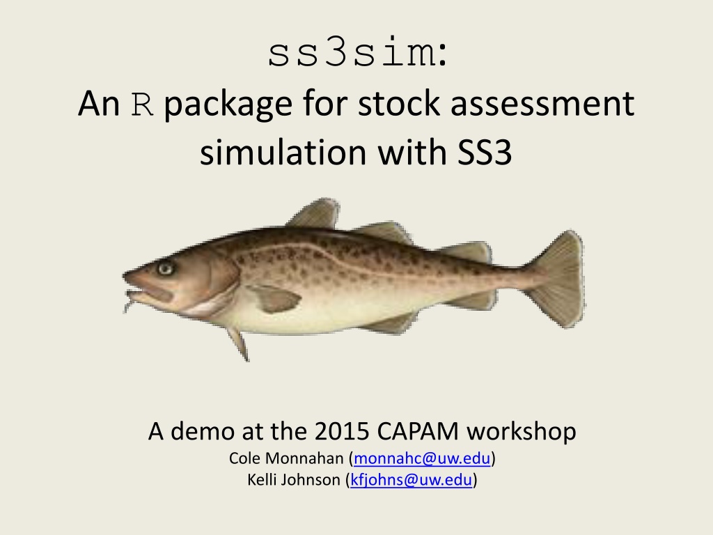
ss3sim: An R package for stock assessment simulation with SS3 A demo at the 2015 CAPAM workshop Cole Monnahan (monnahc@uw.edu) Kelli Johnson (kfjohns@uw.edu)
Outline 1. Install package framework and get familiar with basics 2. Run simple example1 and explore results 3. Modify simulation and rerun 4. Explore process error and data weighting interaction Goal: Learn what the tool is capable of, and whether it may be useful for future projects 1 A set of files accompany this presentation: an R script, case files, and archived results
ss3sim: Big picture What is it? End-to-end simulation framework in R: OM-> Data -> EM-> analysis Software Details Open source, cross platform (Windows, OS X, Linux). Requires: SS3.24o, R >= 3.2.0, r4ss CRAN (http://cran.r-project.org/package=ss3sim) Development version (www.github.com/ss3sim/ss3sim) [recommended] Documentation 1. PLoS One Paper: Introduces the package, describes the philosophy and goals, and details basic functionality with a toy example Vignette and R help files for individual function (?ss3sim , etc.) 2.
ss3sim: Big picture Input files starter control data forecast Output for debugging warning.sso echoinput.sso ParmTrace.sso r4ss SS3 Output with results Report.sso CompReport.sso covar.sso Forecast-report.sso Mirrored Output starter.ss_new control.ss_new data.ss_new forecast.ss_new ss3sim r4ss Adapted from Juan Valero, SS workshop materials
Step 0 Install package with: if(!require(devtools)) install.packages('devtools') devtools::install_github('ss3sim/ss3sim', dependencies = TRUE, build_vignettes = TRUE) Make sure libraries can be loaded <Look at model (OM and EM) files>
Step 1 Run the first example (<look at CPU usage>) <Look at r4ss output> Rerun with more iterations in parallel (<look at CPU usage>) So what is D0-F1-cod ?
ss3sim Cases Conceptually: Mechanism which manipulates model structure In practice:R function arguments to modify OM/EM files The case arguments are passed to internal R functions during execution Cases are specific to a model (e.g., cod ) Two are mandatory: Fishing (F) and Data (D) Some are optional: Which params to estimate, OM process noise, retrospective, etc.
ss3sim Cases Cases sample the data (D) sample_index sample_agecomp smaple_lcomp OM data EM (expected values) fleets;c(2) years;list(seq(76,100, by=2)) sds_obs;list(.2) lognormal samples every 2 years, with =.2
ss3sim Cases Different arguments to the same functions create case numbers fleets;c(2) years;list(seq(76,100, by=2)) sds_obs;list(0.2) D0 High survey effort fleets;c(2) years;list(seq(76,100, by=2)) sds_obs;list(0.4) D1 Low survey effort
ss3sim Scenarios Scenarios: unique combinations of case numbers Data (D) Fishing effort (F) Model (species) Scenario="D0-E0-F0-R0-cod Estimation (E) Retrospective (R)
Step 1 Run the first example (look at CPU usage) Look at r4ss output Rerun with more iterations in parallel (look at CPU usage) So what is D0-F1-cod ? Read in results <Look at scalar and timeseries files>
Result File Structure All Results: ss3sim_scalar.csv ss3sim_ts.csv Scenario1 (D0-F1-cod) Scenario2 (D0-F1-cod) ScenarioN results_scalar_scenario2.csv results_ts_scenario2.csv N Replicate 1 2 bias AdjustBias.DAT AvgBias.DAT log.txt OM EM 1 Nbias (case arguments) SS SS Model files Model files
Collecting Results get_results_all(directory, overwrite_files, user_scenarios) Uses r4ss and extracts from all scenarios in directory Returns: Simulation metrics (scenario, replicate, etc.) OM and EM params and derived quantities Convergence metrics: invertible Hessian, params_on_bounds, max_grad, runtime Stored in two files: ss3sim_scalars for scalar quantities (M, MSY, etc.) ss3sim_ts for time-varying quantities (SSB(y), F(y), etc.)
Plotting Results plot_scalar_points(data, x, y, horiz, horiz2, vert, vert2, color, relative.error, axes.free) Makes liberal use of ggplot and aes_string. Arguments are: x,y: Character columns to plot, where x can be a factor or not horiz, horiz2: Character columns for how to facet by horizontal rows vert, vert2: Character columns for how to facet by vertical columns color: Character column for the color of points or lines (via an aesthetic) relative.error: TRUE/FALSE whether to set ylim=(-1,1) axes.free: TRUE/FALSE whether to set facet y-limits to be free of fixed [see also plot_scalar_boxplot, plot_ts_points, plot_ts_lines, plot_ts_boxplot which have the same syntax and arguments]
Step 2 Goals: Explore how cases are read in and used in R Explore what sample_agecomp does in text editor Task: Add a new case D1 and run new scenarios
Step 3 We won t have time to run it, but let s design and look at the results of a more complicated simulation. Suppose you are interested in the interaction of process error and data weighting: Does process error influence the effect of improperly weighted comp data? How does this change with what params are estimated?
Changing estimated params We will explore 3 cases of estimation1: 1. Neither h nor M estimated (fixed at truth) 2. h estimated 3. M estimated This is done with the change_e function (change estimation).
Process Error Recruitment deviations: Automatically generated (lognormal corrected) OR specified by the user (e.g., miniscule, autocorrelated or heteroskedastic). Recdevs reused across scenarios, such that all iteration 1 s use the same recdevs Use change_tv to add process error to OM parameter.
Step 3: Adding process error Trend added to fishery selex to simulate, e.g., shifts in fishing gear1. 1 parameterized as double normal but setup to be logistic
Observation Error Length, age, CAAL, empirical W@A, mean L@A, and index data, for arbitrary fleets, years, sample sizes Indices: lognormal with specified Compositions: Multinomial or Dirichlet (overdispersed) samples Dynamic binning:programmatically set bin widths. Effective sample size: calculated internally or supplied by user Note: SS3 bootstrapping is NOT used
Step 3: Varying data weights Comp ESS varies from 10% to 1000% for all fleets and years. Index is unchanged, and everything is (as always) unbiased. 1 Growth and many other params fixed for all scenarios
How ss3sim can be used Functions 1. Top level: run_ss3sim 2. Mid level: ss3sim_base, takes cases as function calls instead of text files 3. Low level: separately in custom simulation frameworks Models1 1. Packaged (cod, flatfish, sardine, rockfish, hake) 2. Build your own (see vignette, share it with us!) 1 See github.com/ss3sim/ss3models for more info
Final Thoughts To build a simulation, we recommend: 1. Start with a simple simulation like this one 2. Add complexity slowly, a piece at a time 3. At each step, check individual model files and overall results
Final Thoughts Think of cases as dimensions of a simulation. ss3sim is designed to easily add factorial combinations of cases. Because of the complexity of SS3, it is difficult to produce a generic tool on top of it. It is not designed to test specific real models, instead use it to test general properties of simplified models.
Final Thoughts 1.ss3sim can be used as an end-to-end simulation framework, or just the individual functions for other tasks 2.ss3sim is designed to be reproducible, flexible and rapid. We believe this can be a valuable alternative to custom frameworks. 3. Actively and consistently maintained, and open for new contributors
