Understanding the Essence of Statistics in Decision-Making
Statistics plays a crucial role in making informed decisions by drawing inferences from data collected from a sample to represent a larger population. It involves two key languages: estimation (trust) and hypothesis testing (evidence). By understanding the fundamentals of statistics, managers can navigate uncertainties and anticipate future outcomes based on past data. The process of statistical analysis involves data collection methods and computations to derive meaningful insights for strategic decision-making.

Download Presentation

Please find below an Image/Link to download the presentation.
The content on the website is provided AS IS for your information and personal use only. It may not be sold, licensed, or shared on other websites without obtaining consent from the author. Download presentation by click this link. If you encounter any issues during the download, it is possible that the publisher has removed the file from their server.
E N D
Presentation Transcript
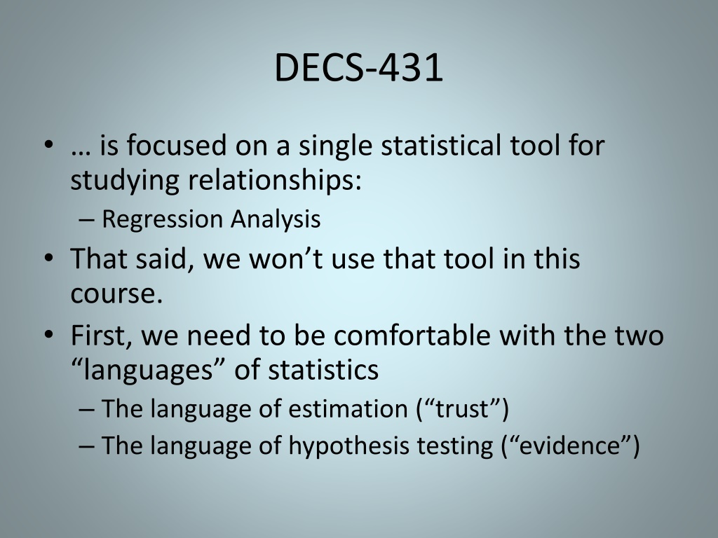
DECS-431 is focused on a single statistical tool for studying relationships: Regression Analysis That said, we won t use that tool in this course. First, we need to be comfortable with the two languages of statistics The language of estimation ( trust ) The language of hypothesis testing ( evidence )
First Part of Class An overview of statistics What is statistics? Why is it done? How is it done? What is the fundamental idea behind all of it? The language of estimation Who cares? Two technical issues, one of which can t be avoided
What is Statistics? Statistics is focused on making inferences about a group of individuals (the population of interest) using only data collected from a subgroup (the sample). Why might we do this? Perhaps the population is large, and looking at all individuals would be too costly or too time-consuming taking individual measurements is destructive some members of the population aren t available for direct observation
Managers arent Paid to be Historians Their concern is how their decisions will play out in the future. Still, if the near-term future can be expected to be similar to the recent past, then the past can be viewed as a sample from a larger population consisting of both the recent past and the soon-to-come future. The sample gives us insight into the population as a whole, and therefore into whatever the future holds in store. Indeed, even if you stand in the middle of turbulent times, data from past similarly turbulent times may help you find the best path forward.
How is Statistics Done? Any statistical study consists of three specifications: How will the data be collected? How much data will be collected in this way? What will be computed from the data? Running example: Estimating the average age across a population, in preparation for a sales pitch.
1. How Will the Data be Collected? Primary Goals: No bias High precision Low cost Simple random sampling with replacement Typically implemented via systematic sampling Simple random sampling without replacement Typically done if a population list is available Covered in next class Stratified sampling Done if the population consists of subgroups with substantial within- group homogeneity Cluster sampling Done if the population consists of (typically geographic) subgroups with substantial within-group heterogeneity Specialized approaches
2. How is the Sample Size Chosen? In order to yield the desired (target) precision (to be made clearer in next class) simple random sampling with replacement sample size of 5
3. What Will be Done with the Data? Some possible estimates of the population mean from the five observations: median (third largest) average of extremes ( [largest + smallest] / 2) sample mean ( x = (x1+x2+x3+x4+x5)/5) smallest (probably not a very good idea)
Weve Finally Chosen an Estimation Procedure! simple random sampling with replacement sample size of 5 our estimate of the population mean will be the sample mean, x = (x1+x2+x3+x4+x5)/5 This will certainly give us an estimate. But how much can we trust that estimate???
The Fundamental Idea underlying All of Statistics At the moment I decide how I m going to make an estimate, if I look into the future, the (not yet determined) end result of my chosen estimation procedure looks like a random variable. Using the tools of probability, I can analyze this random variable to see how precise my ultimate (after the procedure is carried out) estimate is likely to be.
Some Notation population sample size, N size, n mean, sample mean, x standard deviation, , where 2= (xi- )2 / N sample standard deviation, s, where s2= (xi- x)2 / (n-1)
For Our Estimation Procedure, with X Representing the End Result E[ X] = our procedure is right, on average StDev( X) = / n if this is small, our procedure typically gives an estimate close to X is approximately normally distributed (from the Central Limit Theorem)
Pulling This All Together, Heres the Language of Estimation I conducted a study to estimate {something} about {some population}. My estimate is {some value}. The way I went about making this estimate, I had {a large chance} of ending up with an estimate within {some small amount} of the truth. For example, I conducted a study to estimate the mean amount spent on furniture over the past year by current subscribers to our magazine. My estimate is $530. The way I went about making this estimate, I had a 95% chance of ending up with an estimate within $36 of the truth.
For Simple Random Sampling with Replacement I conducted a study to estimate , the mean value of something that varies from one individual to the next across the given population. My estimate is x. The way I went about making this estimate, I had a 95% chance of ending up with an estimate within 1.96 / n of the truth. (And the other 5% of the time, I d typically be off by only slightly more than this.) See Confidence.xlsm .
Theres Only One Problem We don t know ! So we cheat a bit, and use s (an estimate of based on the sample data) instead. And so Our estimate of is x, and the margin of error (at the 95%-confidence level) is 1.96 s/ n .
And Thats It! We can afford to standardize our language of "trust" around the notion of 95% confidence, because translations to other levels of confidence are simple. The following statements are totally synonymous: I'm 90%-confident that my estimate is wrong by no more than $29.61. (~1.64) s/ n I'm 95%-confident that my estimate is wrong by no more than $35.28. (~1.96) s/ n I'm 99%-confident that my estimate is wrong by no more than $46.36. (~2.58) s/ n
Next Why should a manager want to know the margin of error in an estimate? Some necessary technical details (after break) The language of hypothesis testing (evaluating evidence: to what extent does data support or contradict a statement?) (next week) Polling (estimating the fraction of the population with some qualitative property)
The Language of Estimation (for Simple Random Sampling with Replacement) the standard error of the mean (one standard-deviation s-worth of exposure to error when estimating the population mean) s n the margin of error (implied, unless otherwise explicitly stated: at the 95%-confidence level) when the sample mean is used as an estimate of the population mean s . 1 96 n s . 1 a 95%-confidence interval for the population mean x 96 n
Advertising Sales A magazine publishing house wishes to estimate (for purposes of advertising sales) the average annual expenditure on furniture among its subscribers. A sample of 100 subscribers is chosen at random from the 100,000- person subscription list, and each sampled subscriber is questioned about their furniture purchases over the last year. The sample mean response is $530, with a sample standard deviation of $180. s $180 x 1.96 $530 1.96 530 $ $ 36 100 n To whom, and where, is the $36 margin of error of relevance?
Put Yourself in the Shoes of the Marketing Manager at a Furniture Company Part of your job is to track the performance of current ad placements. Each month You apportion sales across all the placements. You divide sales by placement costs. You rank the placements by bang per buck. The lowest ranked placement is at the top of your replacement list, and its ratio determines the hurdle a new opportunity must clear to replace it.
Keep Yourself in the Shoes of the Marketing Manager at the Furniture Company Another part of your job is to learn the relationship between properties of specific ad placements, and the performance of those placements. You do this using regression analysis, with the characteristics of, and return on, previous placements as your sample data. Given the characteristics of a new opportunity (e.g., number of subscribers to a magazine, and how much the average subscriber spends on furniture in a year), you can predict the likely return on your advertising dollar if you take advantage of this opportunity.
One Day, the Advertising Sales Representative for a Magazine Drops By S/he wants you to buy space in this magazine. You ask (among other things), What s the average amount your subscribers spend on furniture per year? S/he says, $530 $36 You put $530 (and other relevant information) into your regression model and it predicts a return greater than your current hurdle rate! Do you jump onboard?
What If the $530 is an Over-Estimate or an Under-Estimate? The predicted bang-per-buck could actually be worse than your hurdle rate! There are many ways to do a risk analysis, and you ll discuss them throughout the program. They all require that you know something about the uncertainty in numbers you re using. At the very least, you can put $494 and $566 into your prediction model, and see what you would predict in those cases. [More generally, (margin-of-error/1.96) is one standard-deviation s-worth of noise in the estimate. This can be used in more sophisticated analyses.]
Sometimes Its Right to Say Maybe If the prediction looks good at both extremes, you can be relatively confident that this is a good opportunity. If it looks meaningfully bad at either extreme, you delay your decision: Gee! This sounds interesting, but your numbers are a bit too fuzzy for me to make a decision. Please go back and collect some more data. If the estimate stands up, and the margin of error can be brought down, I might be able to say Yes.
Practical Issues If it looks good, either now or on a second visit, be sure to get details on the estimation study in writing as part of your deal. (Then you can sue for fraud if you learn the rep was lying.) The risk analysis I ve described is quite simplistic. You can (and will learn to) do better. But you ll need the margin of error for any approach.
General Discussion How would our answer ($530 $36) change, if there were 400,000 subscribers (instead of 100,000)? It wouldn t change at all! N doesn t appear in our formulas. The precision of our estimate depends on the sample size, but NOT on the size of the population being studied. This is WONDERFUL!!!
(Continued) What if there had been only 4,000 subscribers? Still no change. What if there had been only 100 subscribers? Still no change. But wait! Ahhh!! Everything we ve said so far, and the formulas we ve derived, are for an estimation procedure involving simple random sampling with replacement.
Technical Detail #1 If we d used simple random sampling without replacement: E[ Xwo] = , the procedure is still right on average N n StDev( Xwo) = ( / n) : this is somewhat different! 1 N Xwo is still approximately normally distributed (from the Central Limit Theorem)
For Simple Random Sampling without Replacement s N n x 1.96 N 1 n But for typical managerial settings, this extra factor is just a hair less than 1. For example, if N = 100,000 and n = 100, the factor is 0.9995. So in managerial settings the factor is usually ignored, and we ll use s x 1.96 n for both types of simple random sampling.
Technical Detail #2 s 1.96 x In coming up with , we cheated twice! n We invoked the Central Limit Theorem to get the 1.96, even though the CLT only says, The bigger the bunch of things being aggregated, the closer the aggregate will come to having a normal distribution. As long as the sample size is a couple of dozen or more, OR even smaller when drawn from an approximately normal population distribution, this cheat turns out to be relatively innocuous. We used s instead of . This cheat is a bit more severe when the sample size is small. So we cover for it by raising the 1.96 factor a bit.
Very Technical Detail #2 By how much do we lift the 1.96 multiplier? To a number that comes from the t-distribution with n-1 degrees of freedom. This adjusts for using estimates of variability (such as s) instead of the actual variability (such as ), and for deriving these estimates from the same data already used to estimate other things (such as x for ).
Correcting for Using s Instead of t-distribution 95% central probability 12.706 4.303 3.182 2.776 2.571 2.447 2.365 2.306 2.262 2.228 95% central probability 2.201 2.179 2.160 2.145 2.131 2.120 2.110 2.101 2.093 2.086 95% central probability 2.080 2.074 2.069 2.064 2.060 2.042 2.021 2.000 1.980 1.960 degrees of freedom degrees of freedom degrees of freedom 1 2 3 4 5 6 7 8 9 10 11 12 13 14 15 16 17 18 19 20 21 22 23 24 25 30 40 60 120 Note that, as the sample size grows, the correct approximately 2 multiplier becomes closer and closer to 1.96.
A Plethora of Excel Functions! Excel 2010 offers 10(!) different commands for working with the t distribution. T.DIST T.INV T.TEST T.DIST.RT T.INV.2T TTEST T.DIST.2T TINV CONFIDENCE.T T.DIST and T.INV are comparable to NORMDIST and NORMINV (they all focus on left tails). The T. functions both assume a standardized distribution (expected value 0, standard deviation 1). Learn them and you ll be fine. TDIST The older TDIST and TINV commands were inconsistently defined. T.DIST(where, df, TRUE) tells you the probability to the left (below) where you re standing T.INV(cut off, df) tells you where to stand, in order to cut off this much probability to your left (below).
And Whats This Degrees of Freedom Stuff? Every time we make an estimate, we should use a fresh sample. But we don t. So, if we start with n observations, each estimate eats up one degree of freedom. By the time we estimate variability in the data, we re down to n (estimates already made) degrees of freedom. In this course, we re only making one estimate ( x) before we estimate variability (s), so we end up with n-1 degrees of freedom. In other statistical applications, you will make multiple estimates adjust accordingly.
And How Do We Do This? Fortunately, any decent statistical software these days will count degrees of freedom, look in the appropriate t-distribution tables, and give us the slightly-larger-than-1.96 number we should use. In general, just think (your estimate) (~2) (one standard deviation s worth of uncertainty in the way the estimate was made) as in s where the (~2) is determined by the computer x (~ 2) n
Summary Whenever you give an estimate or prediction to someone, or accept an estimate or prediction from someone, in order to facilitate risk analysis be sure the estimate is accompanied by its margin of error: A 95%-confidence interval for the estimated quantity is (your estimate) (~2) (one standard-deviation s-worth of uncertainty inherent in the way the estimate was made) If you re estimating a mean using simple random sampling: s x (~ 2) n In Excel =AVERAGE(range) (-T.INV(0.025,n-1))*STDEV(range)/SQRT(n)
A Regression Example Costs 643 613 673 531 518 594 722 861 842 706 795 776 815 571 673 Mileage 18.2 16.4 20.1 8.4 9.6 12.1 16.9 21 24.6 19.1 14.3 16.5 18.2 12.7 17.5 Age 0 0 0 1 2 1 1 1 0 1 2 2 2 2 0 Make 0 1 0 1 1 0 1 0 0 0 1 1 0 0 1 Maintenance and repair costs ($ in one year): miles driven during year (thousands), age, make (Ford=0, Honda=1).
Estimate mean cost across the entire fleet: 688.87 2.1448 28.84 Univariate statistics Costs 688.866667 16.3733333 111.678663 4.34370919 0.84515425 0.51639778 28.8353068 1.12154089 0.21821789 0.13333333 Mileage Age Make 1 0.46666667 mean standard deviation standard error of the mean 518 673 861 343 8.4 16.9 24.6 16.2 0 1 2 2 0 0 1 1 minimum median maximum range 0.038 -1.189 -0.214 -0.068 0.000 -1.615 0.149 -2.308 skewness kurtosis 15 number of observations t-statistic for computing 95%-confidence intervals 2.1448
Estimate the mean increase in cost per year of age: 73.96 2.2010 17.91 Regression: Costs constant 107.340945 29.6477024 73.9582688 47.4337242 82.0422871 3.91510733 17.9148891 28.9836595 1.3084 7.5726 21.7429% 0.0011% 1.1531 Mileage Age Make coefficient std error of coef t-ratio significance beta-weight 4.1283 0.1677% 0.5597 1.6366 12.9983% 0.2193 48.9578919 84.90% 80.78% standard error of regression coefficient of determination adjusted coef of determination 15 11 number of observations residual degrees of freedom t-statistic for computing 95%-confidence intervals 2.2010
Predict the annual cost for a 1-year-old Ford driven 15,000 miles: 626.01 2.2010 53.25 Prediction, using most-recent regression constant Mileage 107.3409 Age Make 29.6477 73.95827 47.43372 15 coefficients values for prediction 1 0 626.0148 53.25332 48.95789 20.95331 predicted value of Costs standard error of prediction standard error of regression standard error of estimated mean Predict 95.00% 2.2010 confidence level t-statistic residual degr. freedom 11 508.805 743.2245 confidence limits for prediction lower upper 579.8968 672.1327 confidence limits for estimated mean lower upper


")