Understanding Probability Concepts in Statistics
Probability is a fundamental concept in statistics that measures the likelihood of specific events occurring. This summary delves into classical probability, relative frequency concepts, the Law of Large Numbers, and Bayesian or subjective probability. It covers key properties of probability, approaches to calculating it, and how probabilities can be approximated using different methods.
Download Presentation

Please find below an Image/Link to download the presentation.
The content on the website is provided AS IS for your information and personal use only. It may not be sold, licensed, or shared on other websites without obtaining consent from the author. Download presentation by click this link. If you encounter any issues during the download, it is possible that the publisher has removed the file from their server.
E N D
Presentation Transcript
Statistics Session 9 Probability part 2 Ezra Halleck, City Tech (CUNY), Fall 2021
Opening Example revisited Do you worry about your weight? According to a Gallup poll, 45% of American adults worry all or some of the time about their weight. The poll showed that more women than men worry about their weight all or some of the time: 55% of adult women 35% of adult men worry all or some of the time about their weight. Exercise: what approach to probability would this example be associated with? 2
4.2 Calculating Probability (Review) Probability is a numerical measure of the likelihood that a specific event will occur. First Property The probability of an event always lies in the range 0 to 1: ( ) ( ) 0 1 P A Second Property For an experiment, the sum of the probabilities of all simple events (or final outcomes) is always 1: ( ) 1 i P E P E P E 0 1 P E i ( ) ( ) ( ) = + + + = 1 P E 2 3 3
Conceptual Approaches to Probability 1 Classical Probability Two or more outcomes that have the same probability of occurrence are said to be equally likely outcomes. 1 ( ) = P E i Total number of outcomes for the experiment Number of outcomes favorable to Total number of outcomes for the experiment A ( ) P A = Find the probability of obtaining a head for one toss of a coin. 1 head Total number of outcomes 1 2 ( ) = = = .50 P 4
Conceptual Approaches to Probability 2 Relative Frequency Concept of Probability Using Relative Frequency as an Approximation of Probability If an experiment is repeated n times and an event A is observed f times where f is the frequency, then, according to the relative frequency concept of probability: Frequency of SampleSize f n A ( ) P A = = 5
Law of Large Numbers (LLN) Definition Law of Large Numbers If an experiment is repeated again and again, the probability of an event obtained from the relative frequency approaches the actual (or theoretical) probability. 6
Conceptual Approaches to Probability 3 Bayesian or subjective probability is the probability assigned to an event based on judgment, experience, information, and belief. There are no definite rules to assign such probabilities. For the same event, two separate people could have different viewpoints and so assign different probabilities. Largely popularized by the advance in computational technology and methods during the last twenty years. 7
Opening Example revisited Do you worry about your weight? According to a Gallup poll, 45% of American adults worry all or some of the time about their weight. The poll showed that more women than men worry about their weight all or some of the time: 55% of adult women 35% of adult men worry all or some of the time about their weight. Exercise: what approach to probability would this example be associated with? Classical, frequentist or subjective (Bayesian)? 8
Disjoint and non-disjoint outcomes Disjoint (mutually exclusive) outcomes cannot happen at the same time. The outcome of a single coin toss cannot be a head and a tail. A student both cannot fail and pass a class. A single card drawn from a deck cannot be an ace and a queen. Non-disjoint outcomes: Can happen at the same time. A student can get an A in Stats and A in Econ in the same semester.
Intersection of Events Definition Let A and B be two events defined in a sample space. The intersection of A and B represents the collection of all outcomes that are common to both A and B and is denoted by ( ) and A B Important note: Two events are mutually exclusive if and only if their intersection is the empty set. 10
Example 4-14 Consider the following events for one roll of a die: A = an even number is observed= {2, 4, 6} B = an odd number is observed= {1, 3, 5} C = a number less than 5 is observed= {1, 2, 3, 4} Are events A and B mutually exclusive? Are events A and C mutually exclusive? 11
Example 4-14: Solution A = {2, 4, 6}; B = {1, 3, 5}; C = {1, 2, 3, 4} Mutually exclusive events A and B Mutually nonexclusive events A and C Are events A and B mutually exclusive? Since there is no intersection, A and B are mutually exclusive. Are events A and C mutually exclusive? 2 and 4 are in the intersection, so A and B are not mutually exclusive. 12
Example 4-15 Consider the following 2 events for a randomly selected adult: Y = this adult has shopped on the Internet at least once N = this adult has never shopped on the Internet Are events Y and N mutually exclusive? Y and N have no common outcome. Hence, these two events are mutually exclusive. 13
Union of Events Definition Let A and B be two events defined in a sample space. The union of eventsA and B is the collection of all outcomes that belong to either A or B or to both A and B and is denoted by ( or A B ) 14
Addition Rules Union of Two Mutually Nonexclusive Events The probability of the union of two mutually nonexclusive events A and B is ( ) ( ) P A ( ) P B ( ) = + or and P A B P A B Union of Two Mutually Exclusive Events The probability of the union of two mutually exclusive events A and B is ( ) ( ) P A ( ) P B = + or P A B 15
Addition rule : flipping a fair coin 3 times let P(A or B) = P(A) + P(B) P(A and B) = + - 1/8 = 7/8 Note that A or B has only one outcome that is not in it. Namely HTT A = get at least two heads = {HHT, HTH, THH, HHH} B = first flip is tail= {THH,THT,TTH,TTT} A and B = {THH}, so 16
4.3 Marginal Probability, Conditional Probability, and Related Probability Concepts Suppose all 100 employees of a company were asked whether they are in favor of or against paying high salaries to CEOs of U.S. companies. Here is a contingency table or two-way classification of the responses. In Favor 15 4 Against 45 36 Blank Male Female 17
4.3 Marginal Probability, Conditional Probability, and Related Probability Concepts Suppose all 100 employees of a company were asked whether they are in favor of or against paying high salaries to CEOs of U.S. companies. Blank In Favor Male 15 Female 4 Total 19 Against 45 36 81 Total 60 40 100 We have added the marginal totals. 18
Marginal Probability Definition Marginal probability is the probability of a single event without consideration of any other event. In Favor (A) Against (B) Total Blank 60 100 ( ) Male 15 45 60 P M = = .60 Female 4 36 40 40 100 ( ) P F = = .40 Total 19 81 100 19 100 .19 81 100 .81 ( ) ( ) = = P A P B = = 19
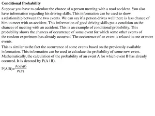
Conditional Probability Definition Conditional probability is the probability that an event will occur given that another has already occurred. If A and B are two events, then the conditional probability of A given B is written as ( ) P A B Read as the probability of A given that Bhas already occurred. 20
Example 4-12 Compute the conditional probability P (in favor | male) for the data on 100 employees given in Table 4.5. In Favor (A) Against (B) Total Blank Male 15 45 60 Female 4 36 40 Total 19 81 100 21
Example 4-12: Solution Number of males who are in favor Total number of males 15 60 ( ) = = = in favor|male .25 P Compare this to the overall rate in favor which 0.19 or 19%. What does this say about men and their view of wage-inequality compared to women? Are men more likely to aspire to reach high-salary positions? 22
Example 4-13 Compute P (female | in favor) the probability of being a woman among those who favor higher salaries for CEO s. In Favor (A) Against (B) Total Blank Male 15 45 60 Female 4 36 40 Total 19 81 100 23
Example 4-12: Solution Number of males who are in favor Total number of males 15 60 ( ) = = = in favor|male .25 P Compare this to the overall rate in favor which 0.19 or 19%. What does this say about men and their view of wage-inequality compared to women? Are men more likely to aspire to reach high-salary positions? 24
Example 4-13: Solution Number of females who are in favor Total number of employees who are in favor 4 .2105 19 ( ) = female|in favor P = = Among those who favor higher CEO pay, 21% are women. 25
Case Study 4-1 Do You Worry about Your Weight? 26
Independence Definition Two events are said to be independent if the occurrence of one does not affect the probability of the occurrence of the other. In other words, A and B are independent events if ( ) ( ) either P A B P A = | ( ) ( ) P B = or P B A | 27
Example 4-16 Are events in favor and female independent? In Favor (A) Against (B) Total Blank Male 15 45 60 Female 4 36 40 Total 19 81 100 4 40 19 100 ( ) ( ) = = = = in favor .19 P in favor female | .1 P Because these two probabilities are not equal, the two events are dependent. Note how being female negatively affects the chance of being in favor 28
Example 4-17 In a survey, 500 adult coffee drinkers were asked whether they drink coffee with or without sugar. Of these 500 adults: 240 are men 175 drink coffee without sugar Of the 240 men: 84 drink coffee without sugar. Are the events drinking coffee without sugar and man independent? 29
Example 4-17: Solution An important skill to develop is to be able to create a contingency table using just partial information. We will also take a frequency contingency table and create a corresponding relative frequency one. men women 169 men 0.312 0.168 0.48 women 0.338 0.65 0.182 0.35 0.52 sugar not sugar 156 84 240 325 175 500 sugar not sugar 91 260 1 175 500 ( ) = = drinks coffee without sugar .35and P 84 240 ( ) = = drinks coffee without sugar man .35 P | Because these two probabilities are equal: the 2 events drinking coffee without sugar and man are independent. 30
