Understanding Conditional Probability and Bayes Theorem
Conditional probability relates the likelihood of an event to the occurrence of another event. Theorems such as the Multiplication Theorem and Bayes Theorem provide a framework to calculate probabilities based on prior information. Conditional probability is used to analyze scenarios like the relationship between driving skills and road accidents. Bayes Theorem helps determine the posterior probability of an event given prior probabilities of related events.
Download Presentation

Please find below an Image/Link to download the presentation.
The content on the website is provided AS IS for your information and personal use only. It may not be sold, licensed, or shared on other websites without obtaining consent from the author. Download presentation by click this link. If you encounter any issues during the download, it is possible that the publisher has removed the file from their server.
E N D
Presentation Transcript
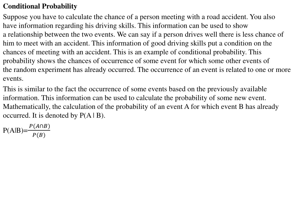
Conditional Probability Suppose you have to calculate the chance of a person meeting with a road accident. You also have information regarding his driving skills. This information can be used to show a relationship between the two events. We can say if a person drives well there is less chance of him to meet with an accident. This information of good driving skills put a condition on the chances of meeting with an accident. This is an example of conditional probability. This probability shows the chances of occurrence of some event for which some other events of the random experiment has already occurred. The occurrence of an event is related to one or more events. This is similar to the fact the occurrence of some events based on the previously available information. This information can be used to calculate the probability of some new event. Mathematically, the calculation of the probability of an event A for which event B has already occurred. It is denoted by P(A | B). P(A|B)=?(? ?) ?(?)
Theorems on Conditional probability Theorem 1 : Let A and B be events of a sample space S of a random experiment. Then, P(S | B) = P(B | B) = 1. Proof: P(S | B) = P(S B) P(B) = P(B) P(B) = 1. [S B shows the outcomes common in S and B equals the outcomes in B]. Theorem 2 : Let A and B be events of a sample S and E is an event of S such that P(E) 0, then P((A B)| E) = P(A | E) + P(B | E) P((A B) | E). Proof: We know P(A B) = P(A) + P(B) P(A B). P((A B) |E) = P((A B) E) P(E) = P((A E) (B E)) P(E). This is the distributive law of union of sets over the intersection. or, P((A B) | E) = [P(A E) + P(B E) P(A B E)] P(E) = [P(A E) P(E)] + [P(B E) P(E)] [P(A B E)] P(E) = P(A | E) + P(B | E) P((A B) | E). If A and B are disjoint events, P(A B) = 0. And, P((A B) |E) = P(A | E) + P(B | E).
Theorem 3: For any two events A and B of a sample space S, P(A B) = P(A). P(B | A), P(A) >0 or, P(A B) = P(B).P(A | B), P(B) > 0. This is the multiplication theorem of probability. Proof: We know that P(B | A) = P(B A) / P(A), P(A) 0. or, P(B|A) = P(A B) P(A) (as A B = B A). P(A B) = P(A). P(B | A). Similarly, P(A B) = P(B). P(A | B). The multiplication theorem of probability can be extended to more than two events. P(A B C) = P(A) . P(B | A). P(C | (A B))
We are quite familiar with probability and its calculation. From one known probability we can go on calculating others. But can we use all the prior information to calculate or to measure the chance of some events happened in past? This is the posterior probability. Bayes theorem calculates the posterior probability of a new event using a prior probability of some events. Bays Theorem: If E1, E2, E3, , Enare mutually exclusive and exhaustive events with P(Ei) 0, (i = 1, 2, , n), then for any arbitrary event A which is a subset of the union of events Eisuch that P(A) > 0, we have P(Ei| A) = [P(Ei).P(A | Ei)] / [ iP(Ei).P(A | Ei)] = [P(Ei).P(A | Ei)] P(A), E1, E2, E3, , Enrepresents the partition of the sample space S.
Proof: A is a subset of the union of Ei, i.e., A Ei, we have, A = A ( Ei) = (A Ei). Also, (A Ei) subset Ei, (i = 1, 2, , n) are mutually disjoint events as Ei s are mutually disjoint. So, P(A) = P[ (A Ei)] = iP(A Ei) = iP(Ei). P(A | Ei). Also, P(A Ei) = P(A). P(Ei| A) or, P(Ei| A) = P(A Ei) P(A) = [P(Ei). P(A | Ei)] [ iP(Ei). P(A | Ei)]. Example 1 Let us consider the situation where a child has three bags of fruits in which Bag 1 has 5 apples and 3 oranges, Bag 2 has 3 apples and 6 oranges and Bag 3 has 2 apples and 3 oranges. One fruit is drawn at random from one of the bags. It was an apple. Let us calculate the probability that the chosen fruit was apple and was drawn from Bag 3. Here, we can calculate the probability of selecting the bags, P(E1) = P(E2) = P(E3) = 1 3. The probability of drawing out of apple from Bag 1, P(A | E1) = 5 8 , from Bag 2, P(A|E2) = 3 9 = 1 3, from Bag 3, P(A | E3) = 2 5. We have to calculate the probability of drawing a fruit given that we have chosen the Bag 3. The probability of drawing a fruit from Bag 3 given that the chosen fruit is an apple is P(E3|A). The Bayes formula helps us to calculate the probability, which is P(E3| A) = [P(E3). P(A | E3)] [P(E1) P(A |E1) + P(E2) P(A | E2) + P(E3) P(A|E3)] P(E3| A) 0= 1 3 2 5 [(1 3 5 8) + (1 3 3 9) + (1 3 2 5)] = (2 15) (163 360) = 48 163.
