Understanding Parametric and Non-Parametric Tests

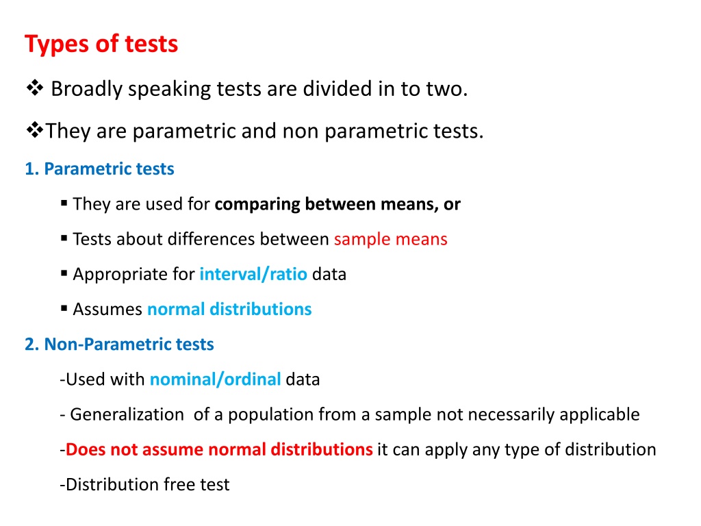
Types of tests Broadly speaking tests are divided in to two. They are parametric and non parametric tests. 1. Parametric tests They are used for comparing between means, or Tests about differences between sample means Appropriate for interval/ratio data Assumes normal distributions 2. Non-Parametric tests -Used with nominal/ordinal data - Generalization of a population from a sample not necessarily applicable -Does not assume normal distributions it can apply any type of distribution -Distribution free test

The R/s b/n Level measurement data treatment, appropriate tests

Parametric Statistics: Analysis of differences Compare Means contents 1. T-test: independent samples 2. T-test: paired samples 3. One-way ANOVA

Compare means 1. Independent T-test Quick facts Number of variables One independent (x) One dependent (y) Scale of variable(s) Independent: categorical with two values (binary) eg. sex Dependent: continuous/scale (ratio/interval)

In many real life situations, we cannot determine the exact value of the population mean We are only interested in comparing two populations using a random sample from each are called sample mean. Such experiments, where we are interested in detecting differences between the means of two independent groups are called independent samples test ( - -- ) The t-test is used to determine whether sample has different means

The independent t-test is a method for comparing the mean of one dependent variable between two (unrelated) groups E.g. sex For example, you may want to see if salary differs between male and female teachers Mean salary among male It tests whether the mean of one sample is different from the mean of another sample Mean salary among female

At the outset the null and alternative hypotheses for the independent samples t-test have to be set up. These take the general form: H0: There is no mean difference between salary of male and female teachers H1: There is a mean difference between salary of male and female teachers

Assumptions 1. Homogeneity of variances. The homogeneity of variance option gives you Levene s test for similar variances Check the significance value (Sig.) for Levene s test. If this number is greater than 0.05 (e.g. 0.09, 0.12, 0.28) then you have not violated the assumption of homogeneity of variance 2. Your dependent variable should be continuous For example: Income, height, weight, number of years of schooling, and so on.

3. Your independent variable should be categorical and unrelated consist of only two groups. Unrelated means that the two groups should be mutually exclusive: no individual can be found in both groups at a time. For example: men vs. women, employed vs. unemployed, and so on.

4. No outliers : An outlier is an extreme (low or high) value. For example, if most individuals have a test score between 40 and 60, but one individual has a score of 96 or another individual has a score of 1, this will distort the test. 5. The distribution should be normal: implies large sample

Summary Research question: Is there a significant difference in the mean salary scores between male and female teachers? What you need: Two variables: one categorical, independent variable (e.g. male/female); and one continuous, dependent variable (e.g. mean salary).

Steps 1. Go to the Menu bar, choose Analyze\Compare Means\Independent-Samples T Test. 2. In the left box, all your variables are displayed. You choose the variable you want to have as your dependent variable and transfer it to the box called Test Variable(s). 3. Then you choose the variable you want as your independent variable and transfer it to the box called Grouping Variable. 4. Click on Define Groups 5. Specify which values the two categories in the independent variable have. 6. Click on Continue. 7. Click on OK.

Interpretation As shown in the figure, farm size is Normally distributed for both genders. As would be expected, it can be seen that the minimum farm size is lower in females than males. Using the descriptive statistics, it can be seen that the mean farm size for females was 0.68 and for males was 0.92 ha. The mean difference in farm size was 0.24 ha (0.92-0.68). This means we are 95% certain that the true population mean difference could be found in between 0.067 and .412. This is also statistically significant difference in mean farm size between males and females at p < 0.01.

2. T-test: paired/matched/correlational Number of variables: Two (reflecting repeated measurement points) Scale of variable(s) : Continuous (ratio/interval) paired samples t-test is used to see the mean difference or change between two measurement points. tests if two measurements within the overall sample are different on the same dependent variable. For example, the improvement of crop production after fertilizer is applied The improvement of statistics result after the course is delivered , etc

For the independent samples t-test, you were supposed to have two groups for which you compared the mean. For the paired samples t-test, you instead have two measurements of the same variable, and you look at whether there is a change from one measurement point to the other. Before intervention and after intervention

Assumptions 1. Continuous variables Your two variables should be continuous (i.e. interval/ratio). For example: Crop production without the use of fertilizer and use of fertilizer (suitable for longitudinal study not cross sectional survey) 2. Two measurement points Your two variables should reflect one single phenomenon, measured at two different time points for each individual. 3. Normal distribution : Use a histogram to check. 4. No outliers

Summary What you need: One set of subjects (or matched pairs). Each person (or pair) must provide both sets of scores. Two variables: two different variables Time 1, Time 2 measured on two different occasions, or under different conditions. What it does: A paired-samples t-test will tell you whether there is a statistically significant difference in the mean scores between Time 1 and Time 2.

Steps 1. Go to the Menu bar, choose Analyze\Compare Means\Paired Samples T Test. 2. In the left box, all your variables are displayed. You choose the variable you want to have as your dependent variable and transfer it to the box called Paired variables. 3. Then you choose the variable you want as your TIME 1 and transfer it to the box called Paired variable and followed to TIME 2. 4. Click on OK.

Output/Step 1 The table called Paired Samples Statistics shows the statistics for the variables. For example, it shows the mean value for each of the two measurement points. In the current example, we see that the mean number of unemployment days is lower in 2003 (mean=8.12) than in 2005 (mean=11.31).

Output/Step 2 The table called Paired Samples Test shows the results from the actual t-test. The first column Mean shows that the mean difference between unemployment days in 2003 and unemployment days in 2005 is -3.190 (this difference is actually just derived from taking 11.31 minus 8.12). The last column Sig. (2-tailed) shows the p-value for this difference. If the p-value is smaller than 0.05, the test suggests that there is a statistically significant difference (at the 5 % level). Thus, here we can conclude that there is a statistically significant difference in mean unemployment days between 2003 and 2005 ( T(4970) = -5.228, p= 0.000).

One-way ANOVA facts Number of variables One independent (x) One dependent (y) Scale of variable(s) Independent: categorical (nominal/ordinal) Dependent: continuous (ratio/interval) One-way ANOVA is similar to independent samples t-test. The difference lies, one-way ANOVA allows you to have more than two categories in your independent variable, E.g. Agro ecology, Marital status. Analysis of Variance, or ANOVA, is testing the difference in the means among 3 or more different samples.

One-way ANOVA will provide you with an F-ratio and its corresponding p-value. The F score shows if there is a difference in the means among all of the groups. The larger the F-ratio, the greater is the difference between groups.

R.A. Fisher An F-ratio equal to or less than 1 indicates that there is no significant difference between groups and the null hypothesis is accepted.

Multiple comparisons ( analyze compare means- One-way ANOVA- post hoc tukey You can do multiple comparison only if you found a significant difference in your overall ANOVA. That is, if the Sig. value was equal to or less than 0.05 (P < 0.05). The post hoc tests will tell you exactly where the differences among the groups occur. Look down the column labelled Mean Difference. Look for any asterisks (*) next to the values listed.

If you find an asterisk, this means that the two groups being compared are significantly different from one another at the p<.05 level. The exact significance value is given in the column labelled Sig.

Assumptions 1. Homogeneity of variances: The homogeneity of variance option gives you Levene s test for homogeneity of variances, which tests whether the variance in scores is the same for each of the groups. Continuous dependent variable 2. Three or more unrelated categories in the independent variable Your independent variable should be categorical With more than two groups. Unrelated means that the groups should be mutually excluded: no individual can be in more than one of the groups. 3. No outliers 4. The distribution is normal. What is the indicator?

H0: There is no mean difference in the continuous variable between three or more categorical variables H1: There is a mean difference in the continuous variable between three or more categorical variables

Steps Using Compare means (both of them are similar) 1. Go to the Menu bar, choose Analyze\Compare Means\One-way ANOVA. 2. In the left box, all your variables are displayed. You choose the variable you want to have as your dependent variable and transfer it to the box called Dependent list. 3. You also choose the variable you want as your independent variable and transfer it to the box called Factor. 4. Go to the box Option. Tick the boxes called Descriptive, Homogeneity of variance test, Means Plot. 5. Click on Continue and then on OK.

Output/Step 2 The table called Test of Homogeneity of Variances shows the results from a Levene s test for testing the assumption of equal variances. The column called Sig. shows the p-value for this test. If the p-value is larger than 0.05, we can use the results from the standard ANOVA test. However, if the p-value is smaller than 0.05, it means that the assumption of homogeneity of variance is violated and we cannot trust the standard ANOVA results.

An F statistic is a value you get when you run an ANOVA test or a regression analysis to find out if the means between two populations are significantly different.

Multiple Comparisons Dependent Variable: farm size Tukey HSD (I) agezone (J) agezone Mean Difference (I-J) Std. Error Sig. 95% Confidence Interval Lower Bound Upper Bound dega woina dega kolla .340* .070 .000 .17 .51 .197* .073 .020 .03 .37 woina dega dega -.340* .070 .000 -.51 -.17 kolla -.143 .073 .122 -.31 .03 kolla dega -.197* .073 .020 -.37 -.03 woina dega .143 .073 .122 -.03 .31 *. The mean difference is significant at the 0.05 level.

Interpretation of multiple comparison Next, we can have a look at the post hoc tests which will tell us where the differences lie. The post hoc test we are using is the Tukey test. These give us comparisons of all the categories with one another. Let s have a look at the box labelled Multiple Comparisons . Once again there is a lot of output but we won t need to look at all of it. In the first column we can see that the mean for the dega group is compared to the mean of the woina dega and of the kolla groups and so on. Of the other columns, we are only going to look at the second, labelled Mean Difference and the fourth, labelled Sig. .

The mean difference does exactly what it says on the tin: it gives us the difference between the means of the different categories. So, for example, we can see that the difference in mean farm size between dega and woina dega is 0.340. This means that the mean farm size of dega is 0.340 times higher than the mean farm size of woinda dega (because it is positive, if it is negative times lower .). The column labelled Sig. gives us our p-values. If we look at this column, we can see that except one the others are significant so it is likely that except one the other groups differ from one another.

For interpretation Strictly consider the following 1. df 2. F value 3. P value 4. Post-hoc comparisons using the Tukey test 5. Compare the mean of the three categories (for example mean and standard deviation from HHs in Dega, Kolla, and Woina Dega

Chi-square Quick facts Number of variables Two Categorical (nominal/ordinal) variables There are two different forms of the chi-square test: a) The multidimensional chi-square test, and b) The goodness of fit chi-square test. .

The multidimensional chi-square test assesses whether there is a relationship between two categorical variables. For example, you want to see if young women smoke more than young men. The variable gender has two categories (men and women) and, in this particular case, the variable smoking consists of the categories: no smoking, occasional smoking and frequent smoking. The multidimensional chi-square test can be thought of as a simple cross table where the distribution of these two variables is displayed:

No smoking Occasional smoking Frequent smoking Men (age 15-24) 85 % 10 % 5 % Women (age 15-24) 70 % 20 % 10 % Assumptions Two or more unrelated categories in both variables Both variables should be categorical (i.e. nominal or ordinal) and consist of two or more groups. Unrelated means that the groups should be mutually excluded: no individual can be in more than one of the groups. For example: low vs. medium vs. high educational level; liberal vs. conservative vs. socialist political views; or poor vs. fair, vs. good vs. excellent health; and so on.

Steps 1. Go to the Menu bar, choose Analyze\Descriptive Statistics\Crosstabs. 2. A small window will open, where you see one big box and three small boxes. In the left box, all your variables are displayed. 3. Here, you choose two variables: one to be the Row variable, and one to be the Column variable. 4. Move your variables to the Row and Column boxes by using the arrows. 5. Click on Statistics. 6. Tick the box for Chi-square. 7. Click on Continue. 8. Tick the box cell, percentage, row

Output The table called Chi-Square Tests shows the results from the chi-square test for the variables TV owned and private house. Here, we look at the row called Pearson Chi-Square and the column Asymp. Sig. (2-sided) to see the p-value for the test. A p-value smaller than 0.05 indicates that there is a statistically significant association (at the 5 % level) between the two variables in the test, whereas a p-value larger than 0.05 suggests that there is not a statistically significant association.

Thank You