Understanding Linear Functions: Slope and Changes in Variables
Linear functions and their relationship to slope are explored in this content. Understanding how changes in the independent variable affect the dependent variable is key to interpreting linear relationships. Through visual representations and explanations, this content illustrates the concepts of linearity, local linearity, slope, and changes in variables, highlighting the significance of these ideas in studying linear functions.
Download Presentation

Please find below an Image/Link to download the presentation.
The content on the website is provided AS IS for your information and personal use only. It may not be sold, licensed, or shared on other websites without obtaining consent from the author. Download presentation by click this link. If you encounter any issues during the download, it is possible that the publisher has removed the file from their server.
E N D
Presentation Transcript
Linear Functions (1,2) 2 3 = slope
Linear Functions 2 3 2 3 Our slope of tells us = slope that a change of x in our independent variable . . . (1,2) x 2 3 . . . elicits a change of x in our dependent variable.
Linear Functions If we increase our x-value from 1 to 4, our y-value will_______. increase decrease 2 3 = slope (1,2)
Linear Functions If we increase our x-value from 1 to 4, our y-value will increase. 2 3 = slope (1,2) If we decrease our x-value from 1 to -5, our y-value will______. increase decrease
Linear Functions If we increase our x-value from 1 to 4, our y-value will increase from 2 to ______. 2 3 = slope (4,4) 2 3 2(3) 3 = = 2 x (1,2) x=3 If we decrease our x-value from 1 to -5, our y-value will decrease from 2 to ___.
Linear Functions If we increase our x-value from 1 to 4, our y-value will increase from 2 to 4. 2 3 = slope (4,4) x= -6 (1,2) 2 3 = 4 x ( 5, 2) If we decrease our x-value from 1 to -5, our y-value will decrease from 2 to ___.
Linear Functions If we increase our x-value from 1 to 4, our y-value will increase from 2 to 4. 2 3 = slope (4,4) (1,2) ( 5, 2) If we decrease our x-value from 1 to -5, our y-value will decreasefrom 2 to -2.
A nice curvy graph = 3 2 2 ( ) f x sin( ) x x x
A nice curvy graph Consider a small portion of the graph . . . . . . . shown here in blue.
Zooming Now zoom in on the blue part of the graph. . .
Zooming In And repeat the process by zooming in on the part colored in pink. . .
Zooming In Keep it up. . .
Typical Behavior = 3 2 2 ( ) f x sin( ) x x x
In general. . . When we zoom in on a sufficiently nice function, we see a straight line.
Local Linearity Informal Definition: A function f is said to be locally linear at x = a, provided that if we "zoom in sufficiently far" on the graph of f around the point (a, f (a)), the graph of f "looks like a straight line." It is locally linear, provided that it is locally linear at every point.
The Derivative of f at a Informal Definition: When f is locally linear at x = a, we have a name for the slope of the line that we see when we zoom in on the graph of f around the point (a, f (a)). This number is called the derivative of f at x = a and is denoted, symbolically by f (a).


