Understanding Estimating and Testing Variances in Statistical Analysis
Estimating and testing variances is crucial in statistical analysis. Population and sample variances are key measures of squared deviations around the mean. Sampling distribution of sample variances, specifically for normal data, follows a Chi-Square distribution. Understanding Chi-Square distributions and critical values aids in analyzing sample variances. The interpretation of Chi-Square critical values provides insights into the relationship between sample and population variances.
- Statistical Analysis
- Estimating Variances
- Testing Variances
- Chi-Square Distribution
- Sampling Distribution
Download Presentation

Please find below an Image/Link to download the presentation.
The content on the website is provided AS IS for your information and personal use only. It may not be sold, licensed, or shared on other websites without obtaining consent from the author. Download presentation by click this link. If you encounter any issues during the download, it is possible that the publisher has removed the file from their server.
E N D
Presentation Transcript
Chapter 6 Estimating and Testing Variances
Introduction Population Variance: Measure of average squared deviation of individual measurements around the mean N = ( ) 2 Y i ( ) 2 = = 2 = 1 i V Y E Y N Sample Variance: Measure of average squared deviation of a sample of measurements around their sample mean. Unbiased estimator of 2 ( 2 1 i S n ) n 2 Y Y i = = 1
Sampling Distribution of S2 (Normal Data) Population variance ( 2) is a fixed (typically unknown) parameter based on the population of measurements Sample variance (S2) varies from sample to sample (just as sample mean does) When the Random Variable Y is normally distributed (that is: Y~N( , )), the distribution of (a multiple of) S2is Chi-Square with n-1 degrees of freedom. (n-1)S2/ 2~ 2with df = n-1
Sampling Distribution of S2 (Normal Data) When Y~N( , ), the distribution of (a multiple of) S2 is Chi-Square with n-1 degrees of freedom. (n-1)S2/ 2~ 2with df = n-1 Properties of Chi-Square distributions: Positively skewed with positive density over (0, ) Indexed by its degrees of freedom (df) Mean = df, Variance = 2(df) Critical Values given in Tables on class webpage and can be obtained with R (along with probabilities, densities, and random samples)
a a 2(a a) df=10 2.156 2.558 3.247 3.940 4.865 15.987 18.307 20.483 23.209 25.188 Chi-Square Distribution Critical Values 0.995 0.990 0.975 0.950 0.900 0.100 0.050 0.025 0.010 0.005 Note that in R, give the LOWER Tail Probability: qchisq(.975,10) = 20.483
Chi-Square Critical Values - Interpretation Consider taking a random sample of n = 11 measurements that are normally distributed with mean and standard deviation Compute the sample variance S2 The quantity X2 = (n-1)S2 / 2 is distributed Chi-Square with n-1=10 df Then P(3.247 X2 = 10 S2/ 2 20.483) = .95 = P(0.325 S2/ 2 2.05) It would be rare for the ratio of the sample variance to the population variance to be less than .325 or greater than 2.05, based on a sample of n = 11 from a normal population
(1-a)100% Confidence Interval for 2 (or ) 1: Choose confidence level (1-a ) 2: Obtain a random sample of n items from the population, and compute s2 3: Obtain 2L and 2U from the table of critical values (or software) for the chi-square distribution with n-1 df 4: Compute the confidence interval for 2 based on the formula below 5: Obtain confidence interval for standard deviation by taking square roots of bounds for 2 2 2 ( ) 1 ( ) 1 n s n s 100 ) a 2 1 ( % CI for : , 2 U 2 L
Statistical Test for 2 Null and Alternative hypotheses 1-sided (upper tail): H0: 2 02HA: 2 > 02 1-sided (lower tail): H0: 2 02 HA: 2 < 02 2-sided: H0: 2 = 02 HA: 2 02 Test Statistic 2 obs ) 1 2 ( n s = 2 0 Decision Rule based on chi-square distribution w/ df = n-1: 1-sided (upper tail): Reject H0 if obs2 U2 = a2 1-sided (lower tail): Reject H0 if obs2 L2 = 1-a2 2-sided: Reject H0 if obs2 L2 = 1-a/22 (Conclude 2 < 02) or if obs2 U2 = a /22 (Conclude 2 > 02 )
Example Mercury Concentration in Albacore Data: n = 34 albacore from eastern Mediterranean (Y = Mercury mg/kg) > mercury [1] 1.007 1.447 0.763 2.010 1.346 1.243 1.586 0.821 1.735 [10] 1.396 1.109 0.993 2.007 1.373 2.242 1.647 1.350 0.948 [19] 1.501 1.907 1.952 0.996 1.433 0.866 1.049 1.665 2.139 [28] 0.534 1.027 1.678 1.214 0.905 1.525 0.763 > mean(mercury) [1] 1.358147 > var(mercury) [1] 0.1942195 > sd(mercury) [1] 0.4407034 Source: S. Mol, O. Ozden, S. Karakulak (2012). "Levels of Selected Metals in Albacore (Thunnus alalunga, Bonaterre, 1788) from the Eastern Mediterranean, Journal Of Aquatic Food Product Technology, Vol. 21, #2, pp. 111-117.
Example Mercury Concentration in Albacore Data: n = 34 albacore from eastern Mediterranean (Y = Mercury mg/kg) qqnorm(mercury, cex=1.5, pch=16, col="red") qqline(mercury, lwd=4, col="blue") shapiro.test(mercury) Shapiro-Wilk normality test data: mercury W = 0.97252, p-value = 0.5344 Normality assumption is reasonable
Example Mercury Concentration in Albacore Data: n = 34 albacore from eastern Mediterranean (Y = Mercury mg/kg) R Computations to obtain 95% CI for 2 and (and output them) s2.mercury <- var(mercury) df.mercury <- length(mercury) - 1 X2.LO <- qchisq(.05/2, df.mercury) X2.HI <- qchisq(1-.05/2, df.mercury) CI.LB <- df.mercury * s2.mercury / X2.HI CI.UB <- df.mercury * s2.mercury / X2.LO var.out <- cbind(s2.mercury, df.mercury, X2.LO, X2.HI, CI.LB, CI.UB, sqrt(s2.mercury), sqrt(CI.LB), sqrt(CI.UB)) colnames(var.out) <- c("Var Est", "df", "X2_L", "X2_U", "Lower", "Upper", "SD Est", "Lower", "Upper") round(var.out, 4) Var Est df X2_L X2_U Lower Upper SD Est Lower Upper 0.1942 33 19.0467 50.7251 0.1264 0.3365 0.4407 0.3555 0.5801
Inferences Regarding 2 Population Variances Goal: Compare variances between 2 populations Parameter: (Ratio is 1 when variances are equal) 2 2 2 1 2 S Estimator: (Ratio of sample variances) 2 2 S 1 Distribution of (multiple) of estimator (Normal Data): 2 2 1 2 2 2 2 2 2 2 S S S S = = = ~ with 1 and 1 F df n df n 1 1 1 1 2 2 2 2 2 1 F-distribution with parameters df1 = n1-1 and df2 = n2-1
Properties of F-Distributions Take on positive density over the range (0 , ) Cannot take on negative values Non-symmetric (skewed right) Indexed by two degrees of freedom (df1 (numerator df) and df2 (denominator df)) Critical values given in Tables on class webpage Quantiles, probabilities, random samples, and densities can be obtained in R (and other Statistical software packages)
Critical Values of F-Distributions Notation: Fa, df1, df2 is the value with upper tail area of a above it for the F-distribution with degrees of freedom df1 and df2, respectively F1-a, df1, df2 = 1/ Fa, df2, df1 (Lower tail critical values can be obtained from upper tail critical values with reversed degrees of freedom) Values given for various values of a, df1, and df2 on various Tables on the class webpage. Note that in R, quantile functions give LOWER TAIL PROBABILITIES: qf(.975,df1,df2) F.025,df1,df2 on a typical F-table
F-Distribution Critical Values (df1 = df2 = 5) upper area middle area lower area 0.25 0.5 0.1 0.8 0.05 0.9 0.025 0.95 0.01 0.98 0.005 0.99 0.001 0.998 upper cv 1.8947 3.4530 5.0503 7.1464 10.9671 14.9394 29.7514 lower cv 0.5278 0.2896 0.1980 0.1399 0.0912 0.0669 0.0336 0.25 0.1 0.05 0.025 0.01 0.005 0.001
F-Distribution Critical Values - Interpretation Consider taking two independent random samples of n1=n2= 6 measurements that are normally distributed with means and common standard deviations = = Compute the sample variances S12, S22 and their ratio F = S12 / S22 The quantity F is distributed F with n1-1=5 numerator df and n2-1=5 denominator df Then P(0.198 F = S12 / S22 5.05) = .90 It would be rare for the ratio of the first sample variance to the second sample variance to be less than .195 or greater than 5.05, based on samples of n1 = n2 = 6 from normal populations with equal variances
Test Comparing Two Population Variances Assumption: the 2 populations are normally distributed 1-Sided Test: : H 2 1 s s 2 2 2 1 2 2 : H 0 A 2 1 2 2 = Test Statistic: F obs Rejection Region: F F a , 1, 1 obs n n 1 2 value: ( ) P P F F obs = 2 1 s s 2 2 2 1 2 2 2-Sided Test: : : H H 0 A 2 1 2 2 = Test Statistic: F obs 2 1 2 2 Rejection Region: ( ) F F a /2, 1, 1 obs n n 1 2 2 1 2 2 or ( ) F F a 1 /2, P F 1, 1 F obs n n 1 2 value: 2min( ( ), ( )) P P F F obs obs
(1-a)100% Confidence Interval for 12/22 Obtain ratio of sample variances Fobs = s12/s22 = (s1/s2)2 Choose a, and obtain: FL = F a , n2-1, n1-1 = 1/ Fa , n1-1, n2-1 FU = Fa , n2-1, n1-1 Compute Confidence Interval: 2 1 2 2 2 1 2 2 s s s s , , F F F F F F L U obs L obs U Conclude population variances unequal if interval does not contain 1
Example Stock Market Returns January Effect = = = = = = January Returns: 36 0.0234 0.0535 36 1 35 n y s df 1 1 1 1 = = = = non-January Returns: 396 0.0535 0.0418 396 1 395 n y s df 2 2 2 2 Treating these months as a random sample of all such months, we can test whether January's volatility (aka variance) differs from the other 11 calendar months. = 2 1 2 2 2 1 2 2 : : H H 0 A 2 2 1 2 2 F ( ( 2 0.0535 0.0418 0.0535 0.0418 ) ( 2 .0144 = s s = = = = = 2 : 1.2799 1.6382 TS F obs 2 ( ) ( ) = = : 0.6415 1. ) 5589 RR F F ( .025,35,395 F .975,35,395 ( P F obs obs ) = 2 min 1.6382 , 1.6382 p P F 35,395 35,395 = ) ) = 2 min .9856,.0144 .0288 Source: C-C. Chien, C-f. Lee, A.M.L. Wang (2002). A note on stock market seasonality: The impact of stock price volatility on the application of dummy variable regression model, The Quarterly Journal of Finance and Economics, 42, pp. 155-162.
Example Stock Market Returns January Effect = = = = = = January Returns: 36 0.0234 0.0535 36 1 35 n y s df 1 1 1 1 = = = = non-January Returns: 396 0.0535 0.0418 396 1 395 n y s df 2 0.0535 0.0418 = 0.6415 2 2 2 2 2 1 2 2 2 0.0535 0.0418 = s s = = = = = 2 1.2799 1.6382 F obs 2 = = 1.7279 F .975,395,35 F F .025,395,35 F a a 1 /2, 1, 1 /2, 1, 1 n n n n 2 1 2 1 2 1 2 2 95% CI for : , F .975,395,35 F F .025,395,35 F obs obs ( ) ( ) 1.6382 0.6415 ,1.6382 1.7279 1.0509 , 2.8306 95% CI for : 1.0509 , 2.8306 1.0251,1.6824 1 2 Note that the having rejected the null hypothesis of equal variances on the previous slide. Confidence Intervals do not contain 1, this is consistent with
Example Stock Market Returns January Effect sms <- read.csv("http://users.stat.ufl.edu/~winner/data/stkmrkt_season.csv") attach(sms); names(sms) jan.group <- ifelse(month==1,1,2) var.test(vwmr ~ jan.group) ## Output > var.test(vwmr ~ jan.group) F test to compare two variances data: vwmr by jan.group F = 1.6379, num df = 35, denom df = 395, p-value = 0.02887 alternative hypothesis: true ratio of variances is not equal to 1 95 percent confidence interval: 1.050714 2.830165 sample estimates: ratio of variances 1.637947
Tests Among k 2 Population Variances Hartley s Fmax Test Must have equal sample sizes (n1= = nk) Test based on assumption of normally distributed data Uses special table for critical values Levene s Test No assumptions regarding sample sizes/distributions Uses F-distribution for the test Bartlett s Test Can be used in general situations with grouped data Test based on assumption of normally distributed data Uses Chi-square distribution for the test
Data Description Experimental units=25 grouped canes, 6 reps per treatment Response: Weight of Juice (lbs) Treatments: 1=Healthy (Control) 2=Top-shoot Borer 3=Stem Borer 4=Top-shoot & Stem Borer 5=Root Borer 6=Termites 7=Stem & Root Borer 8=Root Borer & Termites 9=Top-Shoot & Root Borer 10=Top-Shoot & Stem & Root Borer 11=Top-Shoot Borer & Termites Trt 1 2 3 4 5 6 7 8 9 10 11 n 6 6 6 6 6 6 6 6 6 6 6 mean 42.9167 28.8833 29.7333 17.3500 27.5667 30.2500 26.8167 29.4833 22.0833 25.7167 24.0333 sd 0.8010 1.3438 2.1097 2.6052 3.6811 1.7248 1.5184 2.8541 3.4208 3.9301 4.4840 Source: P.C. Mahalanobis and S.S. Bose (1934). "A Statistical Note on the Effect of Pests on the Yield of Sugarcane and the Quality of Cane- Juice," Sankhya: The Indian Journal of Statistics, Vol.1, #4, pp.399-406.
Hartleys Fmax Test H0: 12= = k2 (homogeneous variances) HA: Population Variances are not all equal Data: smax2 is largest sample variance, smin2 is smallest Test Statistic: Fmax = smax2/smin2 Rejection Region: Fmax F* (Values from class website, indexed by a (.05, .01), k (number of populations) and df (n-1, where n is the individual sample sizes per treatment) Pest Data: Fmax = smax2/smin2 = 4.48402/0.80102 =31.34 F*(.05,11,6-1=5) = 28.2 Reject H0
Levenes Test H0: 12= = k2 (homogeneous variances) HA: Population Variances are not all equal Data: For each group, obtain the following quantities: = = th the measurement from group ( 1,..., 1,..., ) y j i i k j n ij i ~ y = sample median for group ( 1,..., ) i i k i n n k i i z z ij ij ~ y = = = 1 n 1 1 j i j = = = = = = + + ( 1,..., 1,..., ) ... z y i k j n z z n n n . .. i 1 ij ij i k i n i ( ( ) ) k 2 ( ) 1 n z z k . .. i i = = Test Statistic: 1 i F L n k 2 i ( ) z z n k . i ij = = 1 1 i j ( ) = Rejection Region: F F P P F F a , 1, 1, L k n k k n k L
Levenes Test Pest data (lawstat package) pest <- read.table("http://users.stat.ufl.edu/~winner/data/pests_cane.dat", header=F,col.names=c("pest.trt","wt.cane","wt.juice")) attach(pest) install.packages("lawstat") library(lawstat) levene.test(wt.juice, pest.trt, "median") > levene.test(wt.juice, pest.trt, "median") Modified robust Brown-Forsythe Levene-type test based on the absolute deviations from the median data: wt.juice Test Statistic = 1.1536, p-value = 0.3414
Levenes Test Pest data (car package) pest <- read.table("http://users.stat.ufl.edu/~winner/data/pests_cane.dat", header=F,col.names=c("pest.trt","wt.cane","wt.juice")) attach(pest) install.packages( car") library(car) pest.trt <- factor(pest.trt) leveneTest(wt.juice, pest.trt, "median") > leveneTest(wt.juice, pest.trt, "median") Levene's Test for Homogeneity of Variance (center = "median") Df F value Pr(>F) group 10 1.1536 0.3414 55
Bartletts Test General Test that can be used in many settings with groups H0: 12= = k2 (homogeneous variances) HA: Population Variances are not all equal k 2 i i s k = = = = 2 = 1 1 i n n k s i i i = 1 i 1 1 1 k = + 1 C ( ) 3 1 k = 1 i i 1 C k ( ) s ( ) ( = 2 B 2 2 i : ln ln TS X s i = 1 i ) 2 B 2 2 k 2 B : P-value: RR X P X a ; 1 1 k
Bartletts Test Pest Data pest <- read.table("http://users.stat.ufl.edu/~winner/data/pests_cane.dat", header=F,col.names=c("pest.trt","wt.cane","wt.juice")) attach(pest) bartlett.test(wt.juice ~ pest.trt) > bartlett.test(wt.juice ~ pest.trt) Bartlett test of homogeneity of variances data: wt.juice by pest.trt Bartlett's K-squared = 20.883, df = 10, p-value = 0.02192
