Understanding Classification Using Decision Trees
Learn about the concept of classification using decision trees, including the goal of predicting outcomes based on predictors, key ideas like recursive partitioning and tree pruning, and a simple example involving mowers and predictor variables. Explore how decision trees are represented by tree diagrams and how recursive partitioning aids in achieving homogeneity within data subsets.

Download Presentation

Please find below an Image/Link to download the presentation.
The content on the website is provided AS IS for your information and personal use only. It may not be sold, licensed, or shared on other websites without obtaining consent from the author. If you encounter any issues during the download, it is possible that the publisher has removed the file from their server.
You are allowed to download the files provided on this website for personal or commercial use, subject to the condition that they are used lawfully. All files are the property of their respective owners.
The content on the website is provided AS IS for your information and personal use only. It may not be sold, licensed, or shared on other websites without obtaining consent from the author.
E N D
Presentation Transcript
Classification using Decision Trees Suchismit Mahapatra Slides : S. Lazebnik
Decision Trees and Rules Goal: classify/predict an outcome based on a set of predictors. The output is a set of rules Example: Goal: classify a record as will accept credit card offer or will not accept Rule might be IF (Income > $500) AND (Education < 4y) AND (Family <= 2) THEN Class = 0 (non-acceptor) Also called CART, Decision Trees, or just Trees Rules are represented by tree diagrams.
Key ideas Recursive partitioning: Repeatedly split the records into two parts so as to achieve maximum homogeneity within the new parts. Pruning the tree: Simplify the tree by pruning peripheral branches to avoid overfitting.
Recursive Partitioning Pick one of the predictor variables, xi Pick a value of xi, say si, that divides the training data into two (not necessarily equal) portions Measure how pure or homogeneous each of the resulting portions are Pure = containing records of mostly one class Algorithm tries different values of xi, and si to maximize purity in initial split After you get a maximum purity split, repeat the process for a second split, and so on
Simple example: Mowers Goal: Classify 24 households as owning or not owning riding mowers. Predictor variables = Income, Lot Size 6
Income 60.0 85.5 64.8 61.5 87.0 110.1 108.0 82.8 69.0 93.0 51.0 81.0 75.0 52.8 64.8 43.2 84.0 49.2 59.4 66.0 47.4 33.0 51.0 63.0 Lot_Size 18.4 16.8 21.6 20.8 23.6 19.2 17.6 22.4 20.0 20.8 22.0 20.0 19.6 20.8 17.2 20.4 17.6 17.6 16.0 18.4 16.4 18.8 14.0 14.8 Ownership owner owner owner owner owner owner owner owner owner owner owner owner non-owner non-owner non-owner non-owner non-owner non-owner non-owner non-owner non-owner non-owner non-owner non-owner 7
How to split Order records according to one variable, say lot size. Find midpoints between successive values For example. first midpoint is 14.4 (halfway between 14.0 and 14.8) Divide records into those with lotsize > 14.4 and those < 14.4 After evaluating that split, try the next one, which is 15.4 (halfway between 14.8 and 16.0) 8
Categorical Variables Examine all possible ways in which the categories can be split. For example, categories {A, B, C} can be split 3 ways :- {A} and {B, C} {B} and {A, C} {C} and {A, B} With many categories, possible ways to split becomes huge. 9
Measuring impurity - Gini Index Gini Index for dataset A containing m records I(A) = 1 - ?? = proportion of samples in dataset A that belong to class k. I(A) = 0 when all cases belong to same class. Has maximum value when all classes are equally represented (0.50 in binary case). 13
Measuring impurity - Entropy ?? = proportion of samples (out of m) in dataset A that belong to class k. Entropy ranges between 0 (most pure) and log2(m) (equal representation of classes) 14
Impurity and Recursive Partitioning Obtain overall impurity measure (weighted average of individual rectangles). At each successive stage, compare this measure across all possible splits in all variables. Choose the split that reduces impurity the most. Chosen split points become nodes on the tree. 15
Tree Structure Split points become nodes on tree (circles with split value in center) Rectangles represent leaves (terminal points, no further splits, classification value noted) Numbers on lines between nodes indicate # cases Read down tree to derive rule E.g., If lot size < 19, and if income > 84.75, then class = owner 18
Determining Leaf Node Label Each leaf node label is determined by voting of the records within it, and by the cutoff value Records within each leaf node are from the training data Default cutoff=0.5 means that the leaf node s label is the majority class. Cutoff = 0.75: requires majority of 75% or more 1 records in the leaf to label it a 1 node 19
Overfitting - Stopping Tree Growth Natural end of process is 100% purity in each leaf However this can lead to overfitting the data, which ends up fitting noise in the data Overfitting leads to low predictive accuracy of new data. After a certain stage, the error rate for the validation data starts to increase. 21
Pruning CART lets tree grow to full extent, then prunes it back. Intuition is to find that point beyond which the validation error begins to rise. Generate successively smaller trees by pruning leaves. At each pruning stage, multiple trees are possible. Use cost complexity to choose the best tree at that stage. 23
Cost Complexity CC(T) = Err(T) + L(T) CC(T) = cost complexity of a tree Err(T) = proportion of misclassified records = penalty factor attached to tree size (set by user) Among trees of given size, choose the one with lowest CC. Do this for each size of tree. 24
Using Validation Error to Prune Pruning yields a set of trees of different sizes and associated error rates. Two trees of interest: Minimum error tree Has lowest error rate on validation data. Best pruned tree Smallest tree within one std. error of min. error. Adds a bonus for simplicity/parsimony. 25
Regression Trees for Prediction Used with continuous outcome variables. Procedure similar to classification trees. Many splits attempted, choose the one that minimizes impurity. 27
Differences from Classification Trees Prediction is computed as the average of numerical target variable in the data (in CT it is majority vote). Impurity measured by sum of squared deviations from leaf mean. Performance measured by RMSE (root mean squared error). 28
Advantages of trees Easy to use, understand. Produce rules that are easy to interpret & implement. Variable selection & reduction is automatic. Usually do not require feature scaling. Can work without extensive handling of missing data. 29
Disadvantages May not perform well where there is structure in the data that is not well captured by horizontal or vertical splits. Since the process deals with one variable at a time, no way to capture interactions between variables. 30
Summary Trees are both easily understandable and transparent technique for prediction or classification. Essentially, a tree is a graphical representation of a set of rules. Trees must be pruned to avoid over-fitting. Since trees do not make any assumptions about the data, they usually require large number of samples. 31