Understanding Chi-Squared Test in Genetics
Explore the Chi-Squared Test in genetics through practical examples such as Mendel's crosses and pea plant genotypes. Learn how to compare expected and observed data, analyze deviations, and test null hypotheses using statistical methods. Dive into the world of scientific hypothesis testing and make informed decisions based on reliable sampling and accurate assumptions.
Download Presentation

Please find below an Image/Link to download the presentation.
The content on the website is provided AS IS for your information and personal use only. It may not be sold, licensed, or shared on other websites without obtaining consent from the author. Download presentation by click this link. If you encounter any issues during the download, it is possible that the publisher has removed the file from their server.
E N D
Presentation Transcript
Statistical Testing Compare expected and observed Mendel s crosses Theoretical (3:1, 9:3:3:1) Did Mendel get exactly 75 tall plants and 25 short plants? Close deviation due to chance Natural variability of living systems (vs an incorrect hypothesis) Mistakes in counting (vs inappropriate testing) How much deviation is acceptable? Are my underlying assumptions accurate? Is my sampling reliable?
Hypothesis Testing Cross two pea plants with green seeds Yields a population of 880 plants 639 have green seeds 241 have yellow seeds Propose the genotypes of the parents
Scientific Hypothesis Scientific hypothesis Allele for green is dominant to allele for yellow Parent plants were both heterozygous for this trait If this hypothesis is true Predicted ratio of offspring from this cross is 3:1 (based on Mendel s laws) G g Green (G) is dominant Yellow (g) G GG Gg Parents are heterozygous (Gg x Gg) g gG gg Phenotypic ratio is 3:1
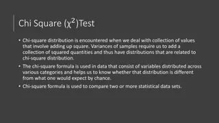
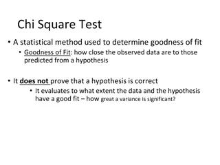
Chi-Square Test Compare observed data with data you would expect to obtain according to a specific hypothesis How much deviation can occur before you conclude something other than chance at work? p = 0.05 2 = (O-E)2 / E O = observed value E = expected value Tests the null hypothesis States that there is no significant difference between the expected and observed result
Null Hypothesis There is no significant difference between your observed pea offspring and offspring produced according to Mendel s laws. Goal: determine if null hypothesis should be rejected or not rejected Use chi-squared
Step 1 Determine number of expected in each category Ratio is 3:1 Total number of observed individuals = 880 Expected numerical values 660 green (3/4 x 880 = 660) 220 yellow (1/4 x 880 = 220)
Step 2 Green Yellow Calculate X2 Observed (o) 639 241 Expected (e) 660 220 Deviation (o-e) -21 21 Deviation2 (d2) 441 441 d2/e 0.668 2.005 X2 = d2/e = 2.673
Step 3 Determine degrees of freedom (df) Number of categories in the problem minus 1 Two categories (green and yellow) 1 df
Step 4 Determine a relative standard to serve as the basis for rejecting the hypothesis Commonly used in biological research: p<0.05 P value probability of rejecting the null hypothesis (no difference between observed and expected) when it is actually true Probability of making an error of falsely stating that there is a significant difference between e and o when there is not a significant difference. p < 0.05 Stating that there is a less than 5% chance of error of stating there is a difference when there actually isn t a significant difference
Step 5 Refer to chi-square distribution table Locate appropriate df (1) Locate the value corresponding to the p value of 0.05
Conclusions If your X2 > distribution table # Reject null hypothesis Conclude observed numbers significantly different from the expected X2 (2.673) is not greater than 3.84 (df=1, p=0.05) Therefore your observed distribution of plants with green and yellow seeds is not significantly different from the distribution that would be expected under Mendel s Laws. Any minor difference -> due to chance Degrees of Freedom (df) Probability (p) 0.95 0.90 0.80 0.70 0.50 0.30 0.20 0.10 0.05 0.01 0.001 1 2 0.004 0.10 0.02 0.21 0.06 0.45 0.15 0.71 0.46 1.39 1.07 2.41 1.64 3.22 2.71 4.60 3.84 5.99 6.64 9.21 10.83 13.82 3 0.35 0.58 1.01 1.42 2.37 3.66 4.64 6.25 7.82 11.34 16.27 4 0.71 1.06 1.65 2.20 3.36 4.88 5.99 7.78 9.49 13.28 18.47 5 1.14 1.61 2.34 3.00 4.35 6.06 7.29 9.24 11.07 15.09 20.52 Nonsignificant Significant


